Design Options to Reduce Conflicts Between Turning Motor Vehicles and Bicycles: Conduct of Research Report (2024)
Chapter: 8 Human Factors Study for Selected Sites
CHAPTER 8
Human Factors Study for Selected Sites
The human factors study explores and validates some design assumptions about bicycle-vehicle interactions, reaction times, cognitive behaviors, and mechanisms of a driving/bicycle simulator, and possibly considers novel designs not currently constructed in the U.S. In the following section, the experimental design methods and protocols, and data collection and reduction methods are detailed. First, all equipment (e.g., software, technology and instrumentation) used to build virtual environments and execute the experimental testing are outlined. The experimental design is then presented, introducing the independent and dependent variables and the corresponding factorial design. The virtual environment development process is then summarized. Afterwards, the chronological structure of protocols for conducting experimental testing is presented. Lastly, the data collection and reduction methods are described.
Research Design and Methods
Equipment
Blender
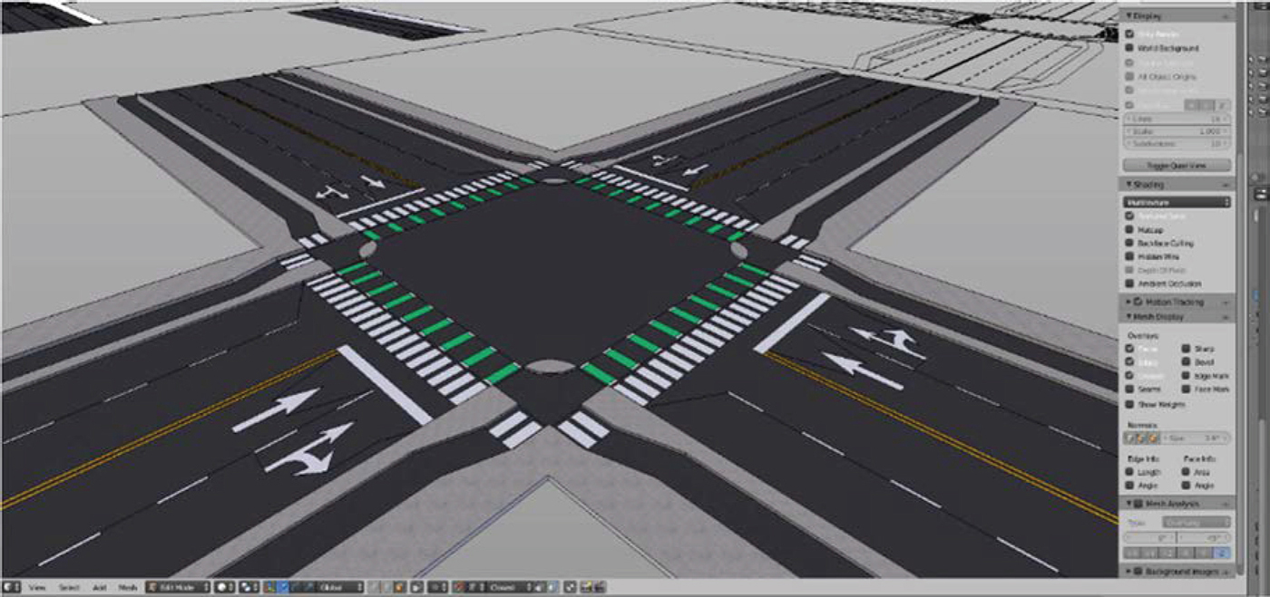
The design and construction of the intersection geometry was completed in Blender (version 2.79), an open-source computer graphics software used for developing and rendering virtual environments. The scope of use was limited to the geometric designs of each intersection surface, including lane configurations, surrounding surfaces (raised curbs and sidewalks) design, pavement markings and surface materials (e.g., asphalt, concrete). A screenshot of the development of the 6-foot offset protected intersections in Blender is shown in Figure 29.
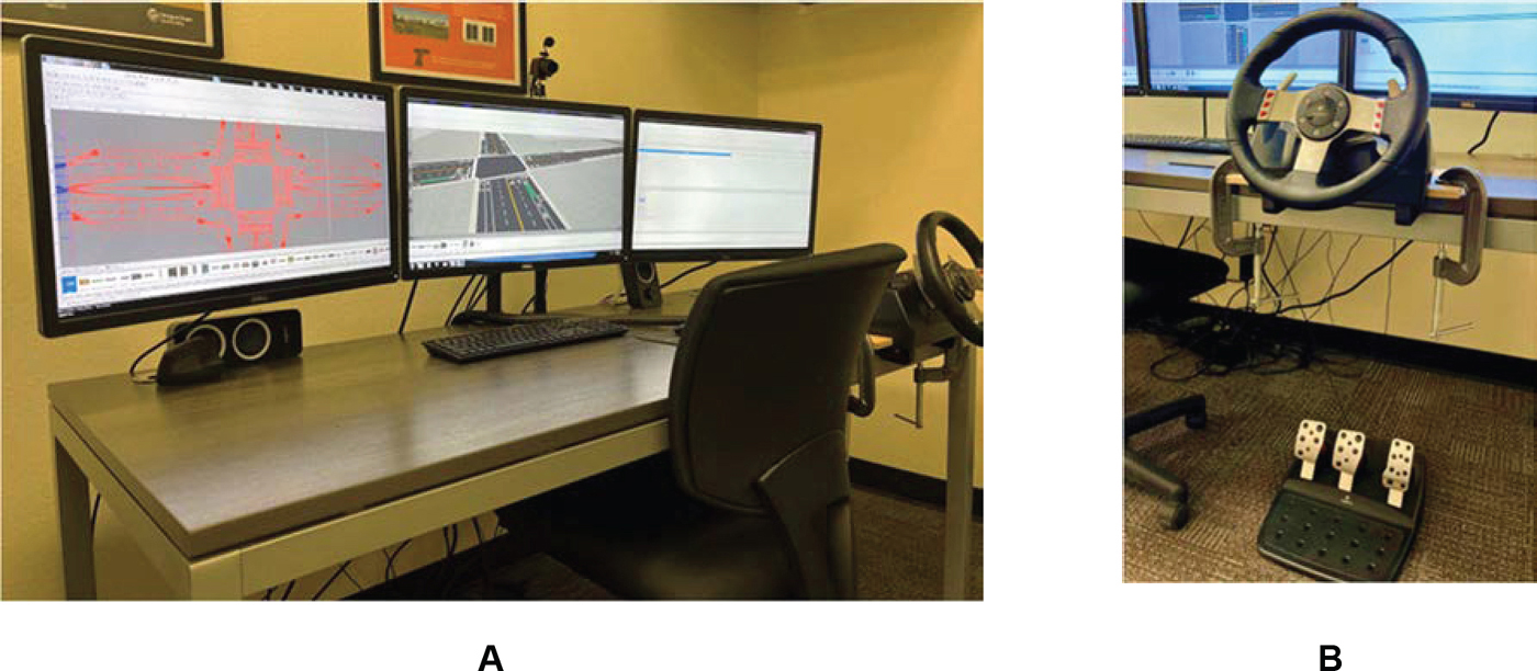
Desktop Driving Simulator
Once the Blender files were completed, they were imported into the desktop driving simulator where Internet Scene Assembler (ISA) was used for the remaining design development steps. As shown in Figure 30A, the desktop driving simulator is composed of three desktop monitors, angled as a tri-fold, a desk-mounted steering wheel and corresponding acceleration and deceleration pedals located on the floor as pictured in Figure 30B. Once imported, these files were scaled and transposed onto programmable surfaces, as displayed on the middle monitor in Figure 30A. The static built environment (e.g., signage, buildings) was then constructed. Next, dynamic roadway elements such as ambient traffic, independent of the experimental design, are integrated and programmed. Lastly, the experimentally controlled variables (i.e., conflicting cyclists), were designed and coded with individual Java scripts and then programmed into the environments. Similarly, the audible route directions, that were provided in real-time, were programmed into the environments using Java scripts.
Full-Scale Passenger Car Driving Simulator
The OSU passenger car driving simulator is a medium-fidelity, motion-based simulator, consisting of a full 2009 Ford Fusion cab mounted above an electric pitch motion system capable of rotating ±4 degrees. The simulator is located in an isolated room designed to mitigate distractions (e.g., sound, light) and conflicting activities during testing. In Figure 31, the passenger car driving simulator is shown, where a researcher is test driving in a previous experimental virtual world.

The vehicle cab is mounted on the pitch motion system with the driver’s eye point located at the center of the viewing volume. The pitch motion system allows for the accurate representation of acceleration or deceleration. Three liquid crystals on silicon projectors (resolution = 1400 by 1050 pixels) are used to project a front view of 180 degrees by 40 degrees. These front screens measure 11 feet by 7.5 feet. A digital light-processing projector is used to display an image on a projector screen located behind the vehicle. This system is designed such that the rear-view mirror reflects the view as it would in a real-world vehicle. Whereas the left and right side-view mirrors have embedded LCD displays. The update rate for the projected graphics is 60 Hz. Ambient sounds around the vehicle and internal sounds to the vehicle are modeled with a surround sound system. The supporting computer system consists of a quad core host running Realtime Technologies SimCreator Software (SimCreator and SimVista Version 2.0, SimObserver Version 4.0 and ISA Version 2.0).
The inside of the vehicle is consistent with a 2009 Ford Fusion with a steering control loading system that accurately simulates the steering torque according to the vehicle speed and steering angle.
SimObserver Data Acquisition System
To provide insight into driver behavior and corresponding performance, real-time kinematic (speed) and trajectory (position) vehicle data were captured using the SimObserver data acquisition system that is integrated into the passenger car simulator. The system also captures multiple camera images of the
participant while driving which are synchronized with the other data feeds. All data is collected at the same rate of 60 Hertz, every 6 seconds.
Head Mounted Eye-tracker
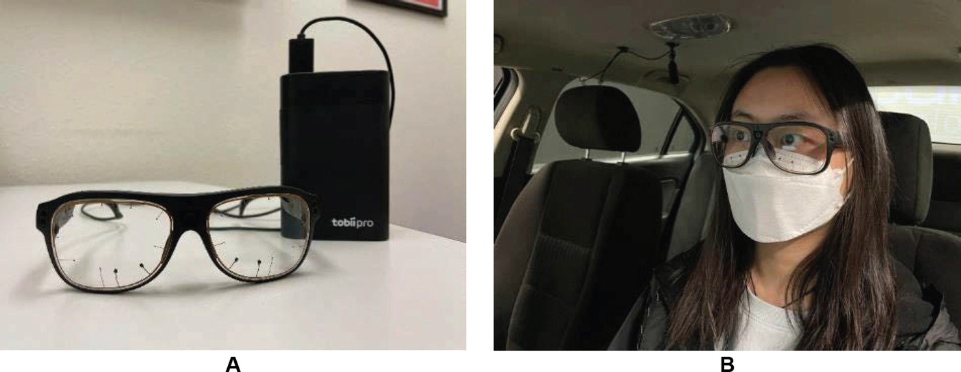
To collect visual attention data, Tobii Pro Glasses 3 eye-tracking glasses were used (Figure 32). It contains a 50Hz or 100Hz sampling rate with an accuracy of 0.6°. Gaze and eye position are calculated using a sophisticated 3D eye model algorithm based on the pupil center corneal reflection technique. The glasses contain eight light sources per lens to illuminate the eye for reflections, and the reflections were captured by the mounted camera for further calculations. The Tobii Pro Glasses 3 uses a wide-angle scene camera that provides wider view and the slippage compensation technology with persistent calibration, which allow user unconstrained eye and head movements throughout the recording (“Tobii Pro Glasses 3”, n.d.).
Via live integration, the recorded data was transferred into the iMotions biometric data processing software for reduction and analysis.
Galvanic Skin Response (GSR) Sensor
A GSR system was used to collect participants GSR and photoplethysmogram (PPG) signals to measure the level of stress. The Shimmer3 GSR+ measures participant GSR and PPG signals:
- GSR data is collected by two electrodes attached to two separate fingers on one hand. These electrodes detect stimuli in the form of changes in moisture, which increase skin conductance and changes the electric flow between the two electrodes. Therefore, GSR data is dependent on sweat gland activity, which is correlated to participant level of stress (Bakker, Pechenizkiy, & Sidorova, 2011).
- PPG signals are collected through photodetectors on skin surfaces (usually a finger or ear-lobe) which measure volumetric variations in blood circulation, giving an accurate and non-intrusive method to monitor participant heart rates (Castaneda, Aibhlin, Ghamari, Soltanpur, & Nazeran, 2018).
Together, GSR and PPG data produce an accurate depiction of participant level of stress. The Shimmer3 GSR+ GSR and PPG sensors attach to an auxiliary input, which is strapped to the participant’s wrist as shown in Figure 33.

Qualtrics
The pre-drive and post-drive surveys were designed and administered through Qualtrics. The initial stages of data cleaning were executed using their internal post-processing functions. The data was then exported to Excel and RStudio for further cleaning, reduction and analysis.
Experimental Design
Independent Variables
The experiment was factorially designed, comprising four independent variables: bike lane configuration (intersection treatment), presence of parallel parking, lateral offset of the bike lane and the proximity of the adjacent cyclist to the intersection when the driver was approaching the point of conflict. Table 37 describes each variable and their corresponding levels. Following, each variable and level is explicitly defined.
Table 73. Independent Variables and Levels
| Variables | Level | Description |
|---|---|---|
| Separation between Vehicle and Bike Lane; Bike Lane Configuration | 1 | None; conventional bike lane |
| 2 | None; pocket/keyhole bike lane | |
| 3 | Partial; mixing zone intersection | |
| 4 | Full; protected intersection with offset bike lane | |
| Relative Location of Bicyclist to Car | 1 | Near; Xcar ≅ Xbike |
| 2 | Far; Xcar > Xbike | |
| Parallel Parking | 0 | No parallel parking |
| 1 | Parallel parking present | |
| Protected Intersection – Offset of Bike Lane | 1 | xoffset = 6 feet |
| 2 | xoffset = 18 feet |
The levels of the first variable, bike lane configuration (intersection treatment), varied by the amount of separation between the cyclist and driver (no, partial and full separation). The first two levels, intersections with a conventional bike lane and a pocket/keyhole bike lane exhibited no physical separation between the cyclist and driver. At the next level, partial separation was tested using the novel mixing zone intersection. For the last level, full separation, a protected intersection was selected, where the physical buffer was 6” raised concrete curbs. In Figure 34, the intersection approaches per bike lane configuration are shown. For simplicity, the infrastructure and surrounding landscapes were removed prior to capturing these images.

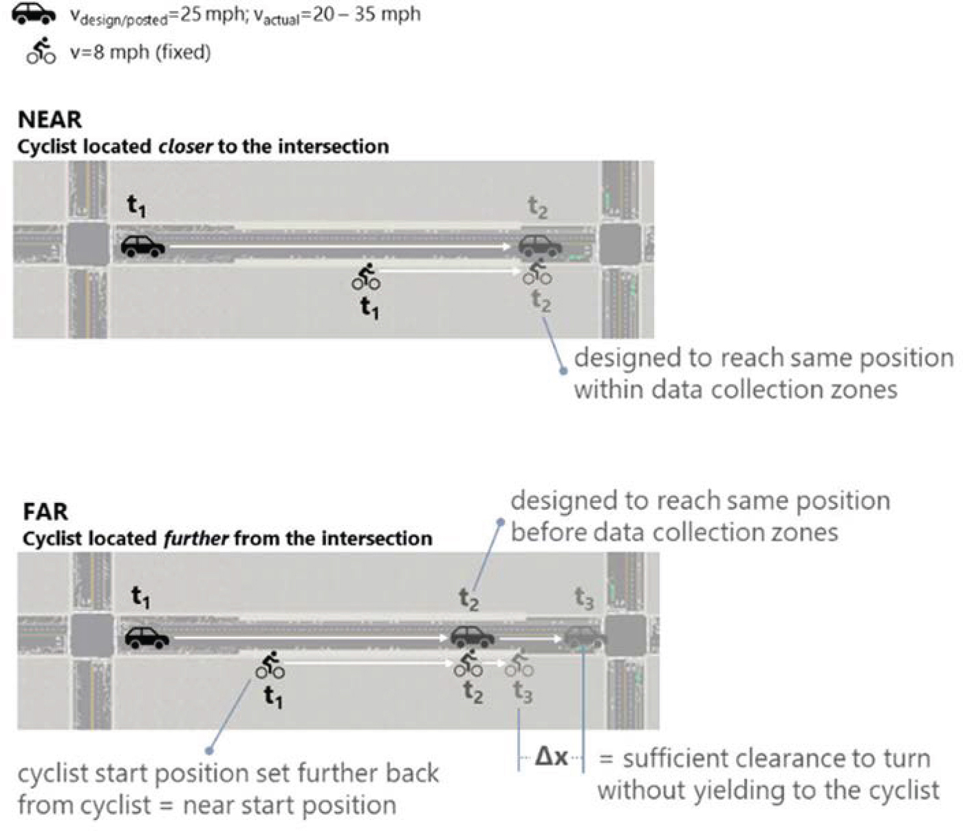
The proximity of the cyclist to the intersection had two levels: closer to the intersection (near) and further from the intersection (far). Figure 35 depicts how this variable was experimentally designed – for the first level, the cyclist start position was designed such that the participant would reach the same position as the cyclist in the data collection zones. This interaction was captured during alpha testing and is shown in Figure 36A. For the second level, cyclist = far, the cyclist start position was located further upstream from the intersection such that the driver would reach the same position before the data collection zones. Similarly, this interaction was captured during alpha testing and is shown in Figure 36B.

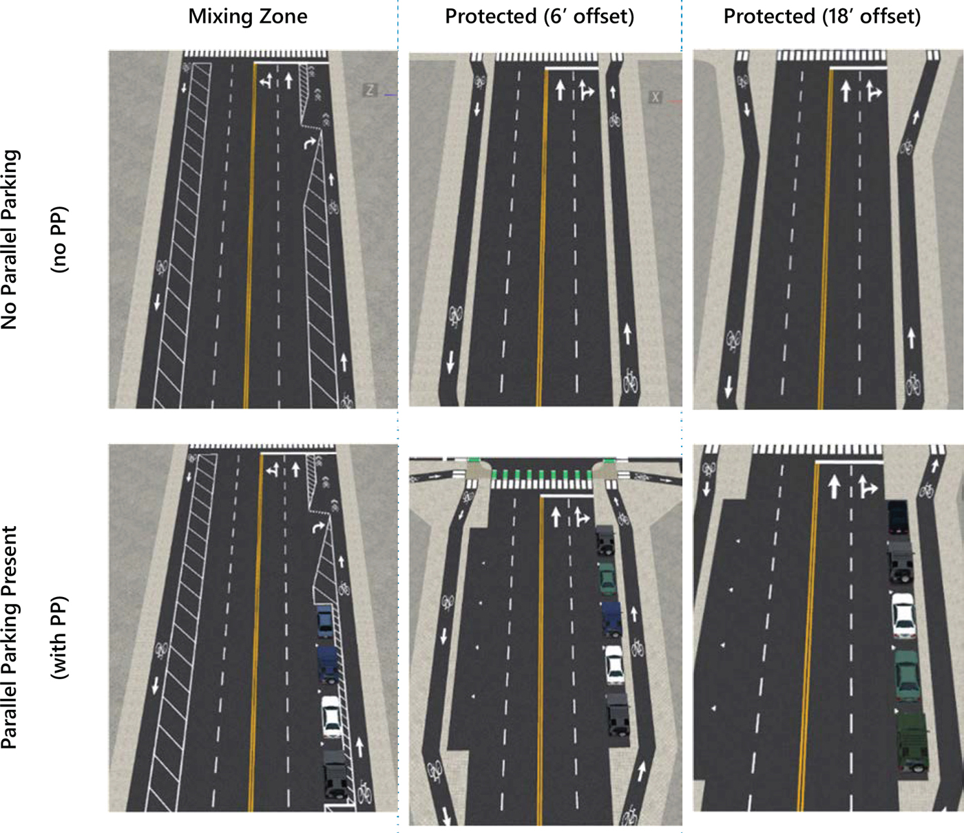
The variable of parallel parking was only applicable to the mixing zone and protected intersections, as the placement of parallel parking at the conventional and pocket/keyhole bike lanes do not directly limit the visibility of cyclists. The three intersection treatments are depicted for each level of parallel parking in Figure 37.
The lateral offset of the bike lane was exclusive to the protected intersections. This independent variable had two levels: 6 feet and 18 feet and are depicted in Figure 38. These two values were selected to represent the upper and lower bounds of the range in lateral offsets observed in literature and existing design.

Vehicle Speed and Positioning Data
Via SimObserver, instantaneous speed and positioning data was recorded (at 60 Hz) for the subject vehicle and the adjacent cyclist. Three variables were selected from the output data to be used for data analysis. The first and second parameters were position and time and were used to map the change in speed and acceleration of the subject with respect to the position on the roadway. The third parameter was the instantaneous speed of the subject, which was used to identify changes in speed approaching an intersection; this parameter was further aggregated at two levels, per data collection zone and per meter. Further, the minimum speeds per data collection zone were obtained using this data to gather insight into participants’ yielding behaviors.
Visual Attention Data
To provide further insight into a driver’s decision-making processes while navigating an intersection and interacting with an adjacent, conflicting cyclist, an eye-tracking system was employed to analyze participants’ visual attention. This biometric instrumentation was used to record participants’ visual attention and reduced to extract the cumulative dwell time (i.e., the total time a participant visually attended to a specific area of interest (AOI), such as the conflicting, adjacent cyclist). The resulting data were reported per participant as the cumulative duration (milliseconds) they spent looking at a given AOI per data collection zone, for all 16 experimental intersections. These results were exported to other types of files, e.g., Excel and RStudio, for statistical analysis to measure participant visual attention during the experiment.
Driver Stress Level Data
GSR biometric instrumentation was used to obtain participants’ peaks per minute (PPM), a metric indicative of stress levels as it provides insight into a driver’s physiological behavior as a response to the roadway environment and other roadway users. To analyze, increases in PPM values are correlated to increased physiological responses to stress. The data collected from the GSR and PPG sensors was wirelessly sent to a host computer running iMotions EDA/GSR Module software, which features data analysis tools such as automated peak detection and time synchronization with other experimental data. The results were exported to other file types (e.g., Excel and RStudio) for reduction and statistical analysis.
Factorial Design
The factorial design of the four independent variables yielded a total of 16 scenarios for experimental testing. The derivation of this count from the independent variables is presented as a matrix of independent variables by treatment type organized in Table 47.
Table 74. Factorial Design Matrix
| Treatment | Parallel Parking | Offset | Cyclist Location | Scenario Count |
|---|---|---|---|---|
| Bicycle Lane (to right of thru lane) | n/a | x n/a | x 2 | = 2 |
| Pocket/Keyhole Bike Lane | n/a | x n/a | x 2 | = 2 |
| Mixing Zone Intersection | 2 | x n/a | x 2 | = 4 |
| Protected Intersection | 2 | x 2 | x 2 | = 8 |
| Σ = 16 |
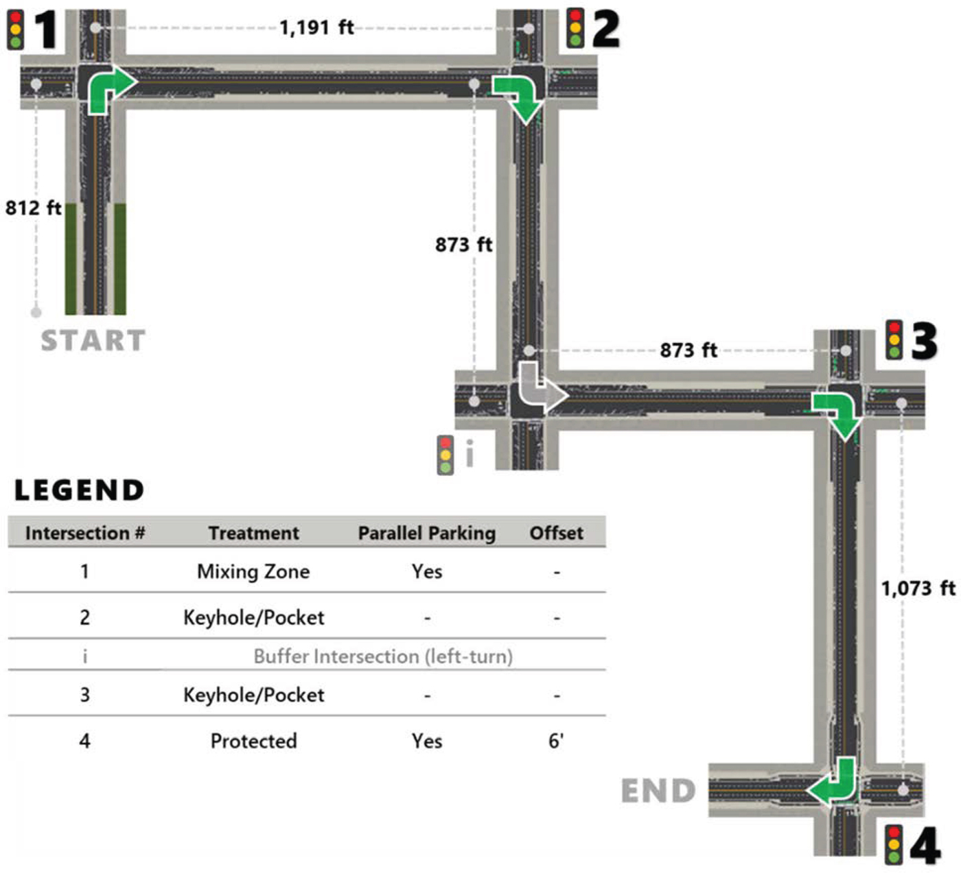
Participants were tasked with maneuvering through and taking a right turn at 16 scenarios. The cumulative duration of consecutively driving through 16 intersections has implications on human performance across time. This is best described by the vigilance decrement, which states that when performing prolonged tasks, humans exhibit a decrease in vigilance overtime. Applied to this experiment, an example of this would be a participant’s decline in accuracy regarding perceiving and measuring the relative proximity of the cyclist to their vehicle. To account for this, the 16 intersections were divided into four virtual worlds (i.e., grids), and subsequently, four separate experimental drives, where participants were provided a two-minute break in between experimental drives. Each scenario was randomly assigned a grid and placement in the respective experimental route. Moreover, the order in which the grids were presented was randomized for each participant. To further add buffer between exposures, an intersection was placed in between the second and third, or third and fourth intersection, where the driver was directed to make a left turn. It should be noted that no data was collected at these left turns. The four grids, their randomly selected scenarios and corresponding variable levels, and the order of presentation are shown in Table 75.
Table 75. Scenario Order by Grid
| Grid | Scenario Order | Treatment | Parallel Parking | Offset | Cyclist Location |
|---|---|---|---|---|---|
| 1 | 1 | Protected | No | 6' | Closer to intersection |
| 2 | Mixing Zone | No | - | Closer to intersection | |
| 3 | Mixing Zone | No | - | Further from intersection | |
| 4 | Protected | No | 18' | Further from intersection | |
| 2 | 1 | Mixing Zone | Yes | - | Further from intersection |
| 2 | Pocket / Keyhole | - | - | Closer to intersection | |
| 3 | Pocket / Keyhole | - | - | Further from intersection | |
| 4 | Protected | Yes | 6' | Further from intersection | |
| 3 | 1 | Protected | No | 18' | Closer to intersection |
| 2 | Conventional | - | - | Further from intersection | |
| 3 | Protected | Yes | 6' | Closer to intersection | |
| 4 | Protected | No | 6' | Further from intersection | |
| 4 | 1 | Mixing Zone | Yes | - | Closer to intersection |
| 2 | Protected | Yes | 18' | Closer to intersection | |
| 3 | Conventional | - | - | Closer to intersection | |
| 4 | Protected | Yes | 18' | Further from intersection |
These grids are composed of two types of tiles, the first being scenario tiles where the tile is composed of one intersection (scenario). These intersections were then connected with connector tiles where these are straight roadway segments that provide seamless transitions between scenarios and their subsequent cross-sectional design. More importantly, these served as a longitudinal and temporal buffer between intersections for drivers. In Figure 39, a top-view perspective of Grid 2 is annotated with the vehicle path followed as described in Table 75.
Dependent Variables
Overall, there are three dependent variables that were obtained from the driver via biometric and simulator equipment: visual attention, speed and GSR.
- Visual Attention: defined as the total fixation duration (TFD), (i.e., the cumulative time a driver spent looking at a specific AOI). There were four AOIs selected, hence, four separate TFDs were measured. These were computed on a zone-level basis; however, their summation was used for data analysis.
- Speed: defined as the vehicle speed profile measured from the starting to ending point of each zone. For data analysis, the average and minimum speeds were calculated per zone.
- Driver Stress Levels: defined as PPM in GSR. These were recorded and analyzed on a per zone basis.
Experimental Protocol
Participant Recruitment
A total of 50 individuals, primarily from the community surrounding Corvallis, OR, were recruited as test participants in the driving simulator experiment. Only licensed drivers with at least one year of driving experience were recruited for the experiment. In addition to driving licensure, participants were required not to have vision prescription higher than five and be physically and mentally capable of legally operating a vehicle. Participants also needed to be deemed competent to provide written, informed consent. Participants were recruited via three primary approaches, flyers shared by the lab’s email listserv, OSU Daily news organization, and word of mouth. During recruitment, prospective participants were not informed of experimental design details that would potentially influence their behavior during the experiment.
Researchers did not screen interested participants based on gender until the quota for either males or females had been reached, at which point only the gender with the unmet quota was allowed to participate. Although it was expected that many participants would be OSU students, an effort was made to incorporate participants of all ages within the specified range of 18 to 75 years. Throughout the entire study, information related to the participants was kept under double lock security in compliance with accepted OSU Institutional Review Board (IRB) procedures (Study Number IRB-2020-0744). Each participant was randomly assigned a number to remove any uniquely identifiable information from the recorded data.
Withholding of Influential Experiment Details
It is important to note that between the recruitment and the completion of the experiment, participants were not informed of any experimental design details that would potentially imposes biases or yield altered behaviors and responses in the pre-drive survey, experimental drives, and post-drive survey.
On the recruitment flyer, contextual information and details regarding the research study were limited to include the project title, Design Options to Reduce Turning Motor Vehicle-Bicycle Conflicts at Controlled Intersections, and a statement generalizing the purpose of the study,
“The purpose of this research study is to improve the safety of bicyclists at intersections.”
Upon the completion of the post-drive survey, the aforementioned experimental design details were shared in response to any questions the participants may have had.
Informed Consent and Compensation
Consent was obtained from all participants prior to beginning any experimental procedures. The IRB approved consent document was presented and explained to the participant upon arrival to the simulator laboratory. This consent document provides an overview of the study, and the objectives of the study. The document also explains the potential risks and research benefits associated with using the simulator. Participants were given $20 compensation in cash for participating in the experimental trial after signing the informed consent document. If participants experienced simulator sickness or they could no longer continue after signing the consent document, they were allowed to leave without penalty.
Pre-Drive Survey
After a participant’s consent was obtained, the pre-drive survey was administered on a computer. This survey asked participants to share basic demographical information (age, gender, highest level of
education, etc.), their prior experience with driving simulators, and their experience as a cyclist (if applicable). Additionally, this survey includes questions from the following areas:
- Vision: Participants were required to report if they wear corrective lenses (glasses) while driving, as the eye tracker contains adjustable lenses up to prescription of five. Participants are required to clearly see the simulation environment and read the visual instructions displayed on the screen. This portion is insured during the calibration drive.
- Simulator Sickness: Participants with previous driving simulation experience were asked about any simulator sickness they experienced. If they have previously experienced simulator sickness, they were encouraged not to participate.
- Motion Sickness: Participants were surveyed about any kind of motion sickness they have experienced in the past. If an individual has a strong tendency towards any kind of motion sickness, they were encouraged not to participate in the experiment.
Calibration Drive
Following the pre-drive survey, participants were first informed of their next task, the calibration drive and its purpose. Participants were then taken into the simulator room, introduced to the passenger car driving simulator and apprised of its degree of personalization regarding mirror angles, steering wheel height, seat setback, and seat height. Next, participants got into the driver’s seat, were asked to buckle their seatbelt and were given the time to make adjustments that would maximize their comfort and driving performance in the experiment. Each participant then completed a calibration drive which was conducted in a large symmetrical grid-based roadway network with ambient traffic. The network was composed of traditional two-lane roads, where a signalized intersection was located at each node. Participants were provided directions in real-time, tasking them with executing left and right-turn maneuvers, like that of the experimental drive.
Overall, the calibration drive took 4-6 minutes and allowed participants to familiarize themselves with the vehicle’s operational mechanics and design, become accustomed to applying the driving task in a full-scale virtual environment and lastly, to confirm if they were prone to simulator sickness. It should be noted that no data was collected during this portion of the experiment, as it was intended to give the participant the chance to become familiar with the equipment and assess their risk of simulator sickness.
Prior to the calibration drive, participants who were not familiar with the concept of simulator sickness were informed of its symptoms and physiological effects. Additionally, participants were encouraged not to ‘push through’ any discomfort or sickness. Moreover, they were ensured that it is okay if they previously identified themselves as not prone to simulator and motion sickness and that they would still be compensated. Following, participants were instructed on what to do if they began to experience simulator sickness – stop driving and place the vehicle into park, and the researcher would enter the simulator room immediately. If a participant reported to feel simulator sickness, their drive was immediately stopped, their participation in the study was terminated and the data collected during their experimental drive was excluded from analysis.
Eye-tracker and GSR Sensor Configuration
Participants were first equipped with the Tobii Pro Glasses 3 eye-tracker. Prior to calibrating the eye-tracking glasses, participants were informed that once calibrated, the glasses cannot be adjusted any time after, including the during the experimental drives. Participants were then allowed to make any last-minute adjustments to the placement of the glasses. Next, participants began the eye-tracking calibration, where they were tasked with looking directly at a target card located 1-2 feet away from their face. This typically took 3-5 seconds.
After the participant was outfitted with the eye-tracking glasses, the participant was equipped with the Shimmer3 GSR sensors. The auxiliary input was placed on the participants’ wrist of choice. If needed, any potentially conflict garments on their wrists, such as smart watches, were removed. The three sensors were each placed at the base of the pointer, middle and index finger. These sensors were wrapped around the participant’s fingers and wrist to ensure secure attachments while optimizing comfort and mitigating any constricting forces on the wrist and fingers.
Experimental Drives
After equipping the participant with the GSR sensor, the researcher briefed the participant on the structure of testing and the tasks required of them. During the experimental drives, the researcher was situated at the operator workstation, located in the control room, where they monitored the participant, vehicle speed and status and simulator room vehicle status on three desktop monitors.
Designed to be completed in <25 minutes, participants executed four experimental drives, with approximately 2-minute breaks between each drive. For each experimental drive, participants were tasked with navigating through and executing right-turns (all on green signals) at four separate signalized intersections and one left-turn at a signalized buffer intersection.
After the participant executed the last and fourth right-turn maneuver in an experimental drive, they were audibly prompted to stop the vehicle and the researcher entered the room to check in on the participant before starting the next experimental drive.
Post-Drive Survey
Following the removal of the biometric equipment, participants were informed of the next and last task, the post-drive survey. The survey was administered on a desktop computer through Qualtrics. Additionally, on a second monitor, participants were provided with a PowerPoint containing aerial images of the simulated intersection designs and their corresponding names. In addition to serving as a complementary resource, the purpose of this PowerPoint was to promote participant’s ability to accurately recall their experiences and to ensure that their responses are submitted for the respective scenario. Participants reported their level of familiarity with each intersection treatment and identified and differentiated between their level of comfort when navigating the intersection when a cyclist was present versus when a cyclist was not present. Participants were provided with the opportunity to submit any thoughts or remarks for each intersection treatment. Further questions surveyed participants on their perceptions and attitudes towards the independent variables and levels, their driving experience exclusive to Oregon and outside of Oregon. After completing the survey, participants were compensated and informed of the study purpose.
From start to finish, the experiment lasted between 50-60 minutes. In summary, the order of tasks completed was as follows: consent process, pre-drive survey, calibration drive, eye-tracker calibration, outfitting of the eye-tracker and GSR sensor equipment, calibration of the eye-tracker glasses, experimental drives, post-drive survey and compensation.
Data Collection & Reduction
For this study, data was collected for three performance measures: the driver’s performance (speed and position), visual attention and stress levels. These were individually reduced and collectively analyzed to describe driver behavior. Vehicle position and speed data was recorded in-real time via SimObserver, a component of the passenger car driving simulator that extracts and reports vehicle kinematic data. Additionally, two types of biometric data were collected in real-time. First, visual attention, was captured using Tobii Pro (eye-tracking) Glasses 3. Second, Shimmer 3 GSR sensors were equipped to participants
to capture their stress levels across each scenario. All three types of data are collectively used to assess driver behavior (e.g., speed, yield decision, stress) when they are navigating the intersection treatments, interacting with adjacent cyclists and maneuvering the conflict points.
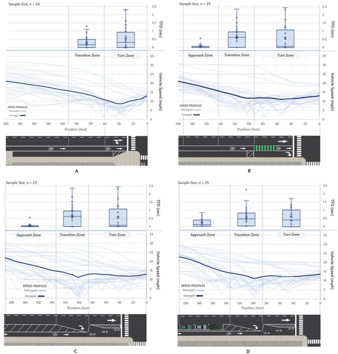
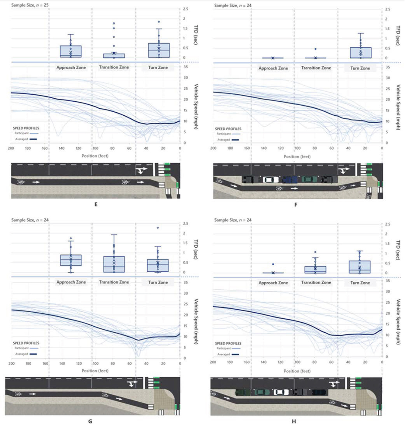
Data Collection Zones
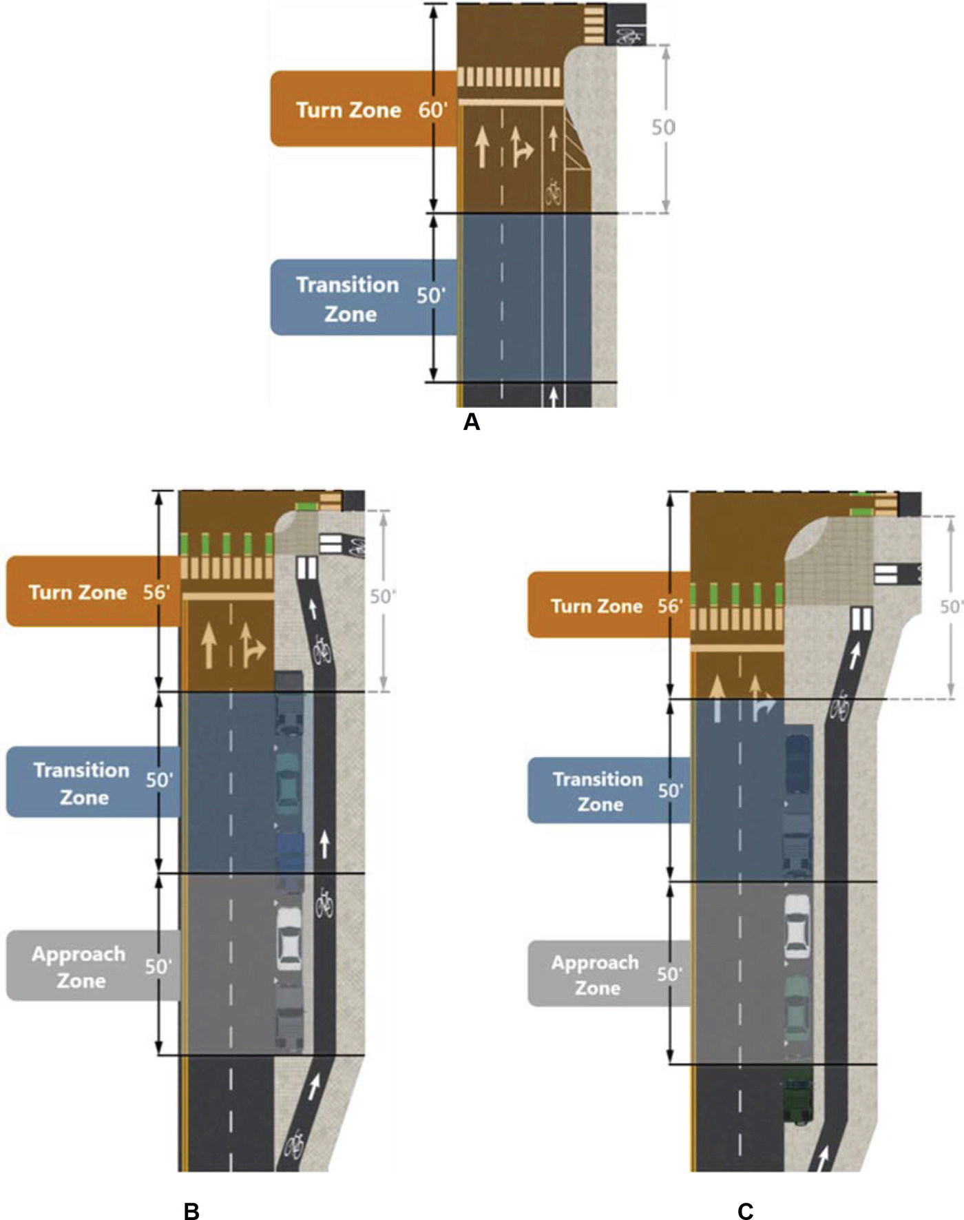
For each scenario, data collection started at a predefined location setback from the stop line and ended immediately after the driver turned right and crossed over the adjacent crosswalk. The distance over which data was collected was further segmented into three zones, defined by setback distances from the reference horizontal. Increasing the complexity and granularity of the traditional data collection methods allowed for more precise analyses that consider the variance in driver behavior and workloads associated with the different stages of navigating and taking a right turn at an intersection. The order of the consecutive zones starting from the furthest upstream of the intersection: approach zone, transition zone, turn zone. The lengths and starting/ending locations of these zones were tailored to the intersection’s geometric design. In Table 76, these locations are documented. Following, these lengths and starting/ending horizontals are annotated on plan view images.
Table 76. Zone Lengths by Scenario
| Zone Type | Approach Zone | Transition Zone | Turn Zone |
|---|---|---|---|
| Conventional Bike Lane | 50' | 50' | 50' |
| Pocket / Keyhole | 50' | 50' | 72' |
| Mixing Zone | 75' | 50' | 70' |
| Protected (6' offset) | 50' | 50' | 56' |
| Protected (18' offset) | 50' | 50' | 56' |
These zone lengths and locations are overlaid on annotated images of the intersections as shown in Figure 40 and Figure 41. For each intersection type and corresponding geometry, the zone locations were designed based on a reference horizontal. This is referred to as the horizontal datum, where the upstream and downstream extent of each zone was setback from this datum.
These horizontals were located at the first vehicle-bicyclist conflict point during the turning maneuver, and hence served as either the beginning of the turn zone, or the end of the data collection (and turn zone). It should be noted that data collection (end of turn zone) was located immediately after the adjacent crosswalk of the lane drivers are turning into.
For the pocket/keyhole bike lane and mixing zone scenarios, their distinct upstream (from the stop line) merge/yield points were selected to serve as their horizontal datums. The zone bounds and lengths are provided in Figure 40.
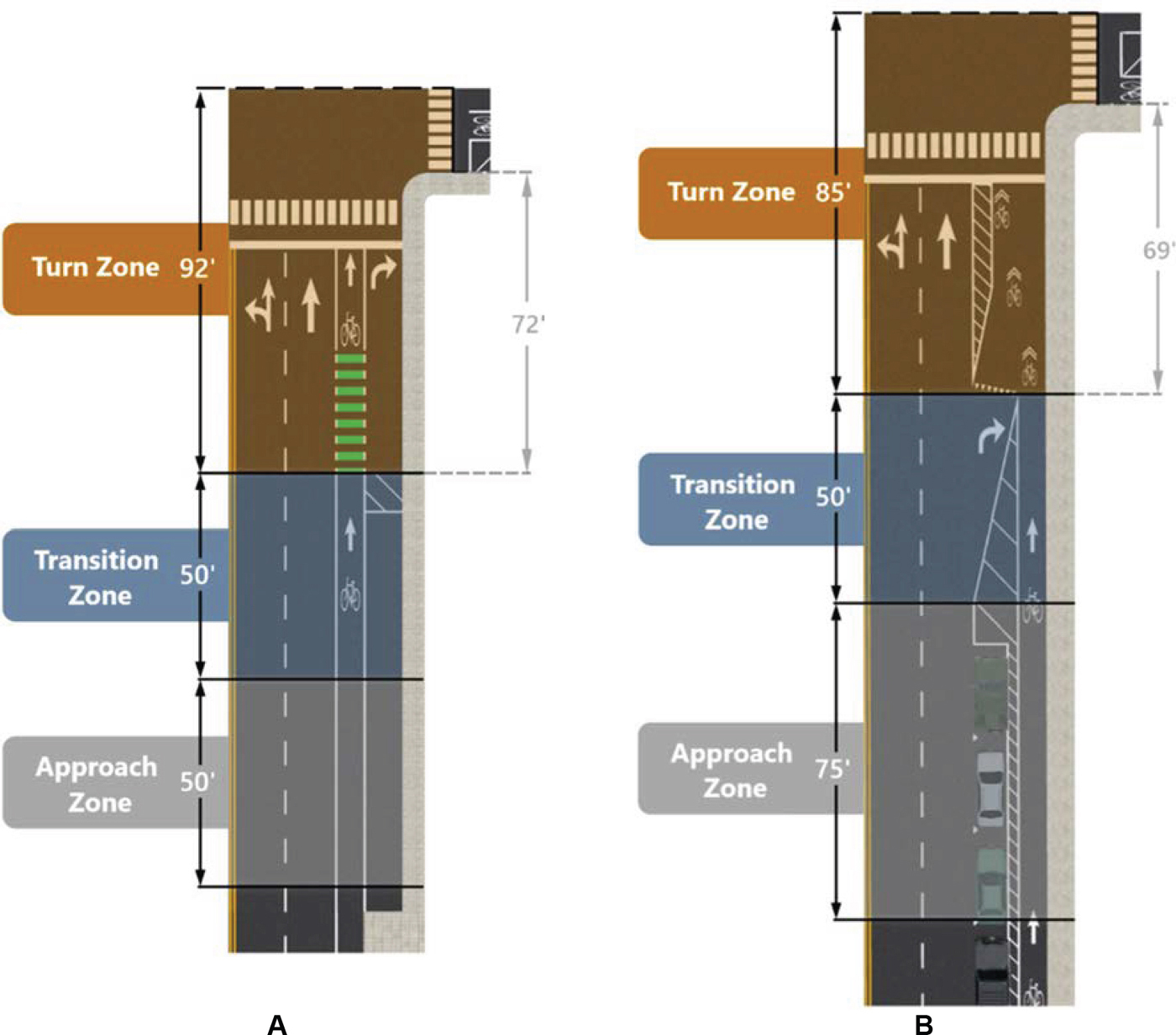
For the conventional bike lane and protected intersection, the positioning of their datums were represented by the horizontal created by the sidewalk curb perpendicular to their initial direction of travel. By design, these horizontal datums corresponded to the end of the turn zone. In Figure 41, these are depicted by the light grey annotation on the right-side of each diagram.
Data Reduction Methods
Simulator Data
The simulator data was used to determine drivers’ speed and position and was obtained from the SimObserver platform. The data file was processed through computer software, (i.e., Data Distillery) and presents the combination of the video data and numerical and graphical outputs. This data was then exported to Excel or RStudio for further data cleaning and reduction. The simulator data was output for each experimental drive (for an individual participant) and consisted of the instantaneous speeds, their corresponding position (X, Y and Z coordinates) and time-stamps relative to each grid. These were then aggregated across scenarios and zones to calculate average and minimum speeds.
Eye-Tracking Data
The visual attention data was wirelessly transmitted to iMotions data reduction software on the host computer. This data was collected and reduced on a per-zone basis across all scenarios. These videos varied in length as driver behavior varied between participants and independent variable levels. Researchers manually coded the starting and ending points of each zone, as their signal values were recorded with the visual attention data. Next, researchers examined each scenario and zone, and coded polygons over the AOIs, uniquely named based on the AOI, scenario and zone. Further, the boundaries were adjusted every 100 milliseconds fit the AOI frame-by-frame. The four AOIs defined in the experimental design were the (1) adjacent, conflicting cyclist, (2) pavement markings, (3) parallel parked vehicles and (4) rear-view and right side-view mirrors. Across all data collection zones, by each video frame, polygons were drawn over the field of view spanned by the AOI. These polygons were resized or moved between frames to ensure the polygon accurately spanned the visual space corresponding to the AOI. Secondly, these adjustments accounted for uncontrolled, continuous head movements that affected the participant’s horizontal body reference and corresponding normal line of sight to the AOI. For a single video frame, if a participant’s gaze fell within the perimeter of an AOI’s region, then the participant was considered to have looked at the AOI for 100 milliseconds. Per data collection zone, and for each AOI, the cumulative number of video frames where the participant’s gaze fell within that AOI’s region equated the TFD – the amount of time spent looking at that specific AOI.
GSR Data
The data collected by the GSR equipment (GSR data and PPG signal) was wirelessly sent to the host computer running iMotions EDA/GSR Module software, which feature data analysis tools such as automated peak detection and time synchronization with other experimental data. The data was reduced to GSR PPM to control the natural variation between participants’ peak measures. The PPM was reported on a per-zone basis. These values were analyzed at the zone-level and at the scenario-level, as the maximum PPM measured across the scenario.
Pre- and Post-Drive Surveys
The data collected from the pre- and post-drive surveys were directly exported from Qualtrics to Excel to be further cleaned, reduced and analyzed.
Human Factors Study Data Analysis & Results
Introduction
In the following section, a comprehensive summary of results is provided. The in-experiment design measures are reported individually (visual attention, speed, GSR). The presentation of these results provides context and reason for the post-experiment survey results to follow.
Participant Sample
Sample Size
A total of 50 participants were recruited and completed the pre-drive survey. As shown in Table 77, the sample size per gender and their corresponding average age (AA) and standard deviation (SD) is as follows: 21 females ( = 36.9, σ = 18.5) (AA=36.9, SD=18.5) 27 males (AA=32.3, SD=11.8) and two non-binaries (AA=21.0, SD=1.41). All participants executed the practice trial, where they were introduced to the driving simulator and given the time and space to familiarize themselves with the vehicle and practice driving in a virtual environment, and experience to ensure they did not experience simulator sickness. Of these 50 participants, 10 were unable to start or complete the experimental driving portion (Table 78). The remaining 40 participants formed the usable dataset for analysis and hence is referred to as the sample moving forward, excluding all participants who experienced simulator sickness.
Table 77. Gender and Age Distribution
| Category | Female | Male | Non-Binary | Total |
|---|---|---|---|---|
| Sample Size | 21 | 27 | 2 | 50 |
| Average Age | 36.9 | 32.3 | 21 | 33.7 |
| Standard Deviation | 18.5 | 11.79 | 1.41 | 15.04 |
Table 78. Participant Sample Size
| Category | Female | Male | Non-Binary | Total |
|---|---|---|---|---|
| Total Participated | 21 | 27 | 2 | 50 |
| Sim Sickness | 3 | 6 | 1 | 10 |
| Completed Testing | 18 | 21 | 1 | 40 |
Data Quality
The data from the sample (n=40) was collected, reduced and used for data analysis. Of these participants, most data were successfully recorded to the highest quality. However, there were instances where technical failures occurred with the data collection equipment. In Table 79, these are noted.
| Category | Eye Tracker | Sim Observer | GSR |
|---|---|---|---|
| Total Tested | 40 | 40 | 40 |
| Collected (usable) | 28 | 38 | 38 |
| Not Collected | 12 | 2 | 2 |
While the analyzed samples were less than the original sample size of 50 participants, the resulting samples remain sufficient in size for statistical analyses to be conducted. According to a recently published study, which investigated sample sizes for driving simulator experiments used to evaluate the safety of freeways, the convergence elbow of the mean squared error curves prove for an acceptable sample size to be 30 participants (Wang et al., 2023). In 2019, Barlow et. al. similarly conducted a simulator study with 54 participants initially recruited and had a final sample size of 30 participants and were still able to perform statistical analyses and draw statistically grounded conclusions (Barlow et al., 2019). Further, many peer-reviewed driving simulator studies have sample sizes of 30 or fewer participants (Donmez et al., 2006; Milloy and Caird, 2009; Owens et al., 2011; Warner et al., 2017).
Pre-Drive Survey
The goal of the pre-drive survey was to collect basic demographic information and data regarding their experience with biking in terms of their self-reported cyclist classification on the Geller Scale and their trip types. In the following section, these results are presented.
Demographics
In Table 80, the demographics of the sample population are presented. Of the participants (n=40), 18 identified as female (45%), 21 identified as male (52.5%) and one identified as non-binary (2.5%). Across the sample, the AA was 33 years, the median age was 26 years, and the SD was 15 years. The AA of the female participants was 36 years, 30 years for male participants and 22 for non-binary participants.
| Variable | Response | Count | Percentage |
|---|---|---|---|
| Gender | Female | 18 | 45.0% |
| Male | 21 | 52.5% | |
| Non-binary | 1 | 2.5% | |
| Age | 18-24 | 17 | 42.5% |
| 25-34 | 8 | 20.0% | |
| 35-44 | 6 | 15.0% | |
| 45-54 | 5 | 12.5% | |
| 55-64 | 2 | 5.0% | |
| 65-74 | 2 | 5.0% | |
| Ethnicity | Asian | 5 | 12.5% |
| Black or African American | 1 | 2.5% | |
| Hispanic or Latino/a | 1 | 2.5% | |
| White or Caucasian | 30 | 75.0% | |
| Other | 1 | 2.5% | |
| Prefer not to answer | 2 | 5.0% | |
| Annual Household Income | $200,000 or more | 3 | 7.5% |
| $100,000 to less than $200,000 | 8 | 20.0% | |
| $75,000 to less than $100,000 | 6 | 15.0% | |
| $50,000 to less than $75,000 | 4 | 10.0% | |
| $25,000 to less than $50,000 | 7 | 17.5% | |
| Less than $25,000 | 9 | 22.5% | |
| Prefer not to answer | 3 | 7.5% | |
| Highest Level of Education Completed | Associates | 3 | 7.5% |
| Four-year degree | 7 | 17.5% | |
| Master's degree | 14 | 35.0% | |
| PhD degree | 2 | 5.0% | |
| Some college | 14 | 35.0% |
Cycling Experience
Following the demographic questions, participants were asked about their experience with cycling. In Table 81, the questions asked, and their corresponding results are shown. Across the sample, 57.5% participants identified as “enthused and confident” cyclists (n=23). Moreover, 77.5% of the participants reported to bike on roadways for exercise, recreation, or commuting/running errands (n=31).
Table 81. Sample Cycling Experience (Self-reported)
| Question | Response | Count | Percentage |
|---|---|---|---|
| What type of cyclist would you classify yourself as? Geller Scale was provided with definitions |
Strong and fearless | 7 | 17.5% |
| Enthused and confident | 23 | 57.5% | |
| Interested but concerned | 8 | 20.0% | |
| No way, no how | 2 | 5.0% | |
| Do you bike on roadways for exercise, recreation, and/or commuting/running errands? | Yes | 31 | 77.5% |
| No | 9 | 22.5% | |
| If selected ‘Yes' in previous question, What activities do you use your bicycle for? (Check all that apply) | Recreation | 27 | 87.1% |
| Commuting | 27 | 87.1% | |
| Exercise | 21 | 67.7% |
It should be noted that the participant sample was over representative of the two most confident cyclist types and under representative of the two least confident cyclist types in comparison to the general population (GP) documented by Dill and McNeil in 2016. In their research, Dill and McNeil conducted a survey across 50 of the largest U.S. Metropolitan cities, with a 3,000 adult sample size and found that across the population, only 7% identified as “Strong and Fearless”, 5% identified as “Enthused and Confident”, 51% identified as “Interested but Concerned”, and 37% identified as “No way, no how” (Dill and McNeil, 2016). In comparison, the first two cyclist types (higher levels of confidence) were overrepresented in the 40-person sample (Strong and Fearless: Sample = 17.5% vs. GP = 5%; Enthused and Confident: Sample = 57.5% vs. GP = 7%). Correspondingly, the remaining two cyclist types (lower levels of confidence) were underrepresented in the 40-person sample (Interested but Concerned: Sample = 20% vs. GP = 51%; No Way, No How: Sample = 5% vs. GP = 37%).
In the following three subsections, the distribution of data from the in-drive data measures (visual attention, speed and GSR) are presented using box and whisker plots. For each data measure, results from all scenarios are presented together.
Visual Attention
Visual attention data was recorded using the iMotions Tobii Glasses 3 and reduced through the iMotions software. As mentioned in the methods, the AOI polygons were drawn for each participant and when their gaze entered the polygon and fixated within the polygon for more than 10 milliseconds, that segment of time was marked as the participant fixating on that specific AOI. The performance measure representing participants’ visual attention on a specific AOI is called the TFD in seconds, which is calculated as the cumulative time elapsed during every fixation across all three zones (approaching, transition and turning).
The results are visualized using box and whisker plots showing the distribution of the TFD across the participant sample, individually separated by AOI. Per AOI, these distributions are sorted and plotted by scenario and cyclist location. For each AOI, results from all scenarios are presented in a single plot, with the corresponding descriptive statistics (average, median, SD) organized in a table following each box and whisker plot.
AOI: Cyclist
Figure 42 shows the distribution, by scenario, of the cumulative time a participant spent visually focusing on the cyclist (from the start of the approach zone to the end of the turn zone). The data is further distinguished by the relative location of the cyclist. The corresponding descriptive statistics are organized in Table 82. Considering the size of data presented, the results are further separated and presented by the most distinct variable, the relative location of the cyclist.
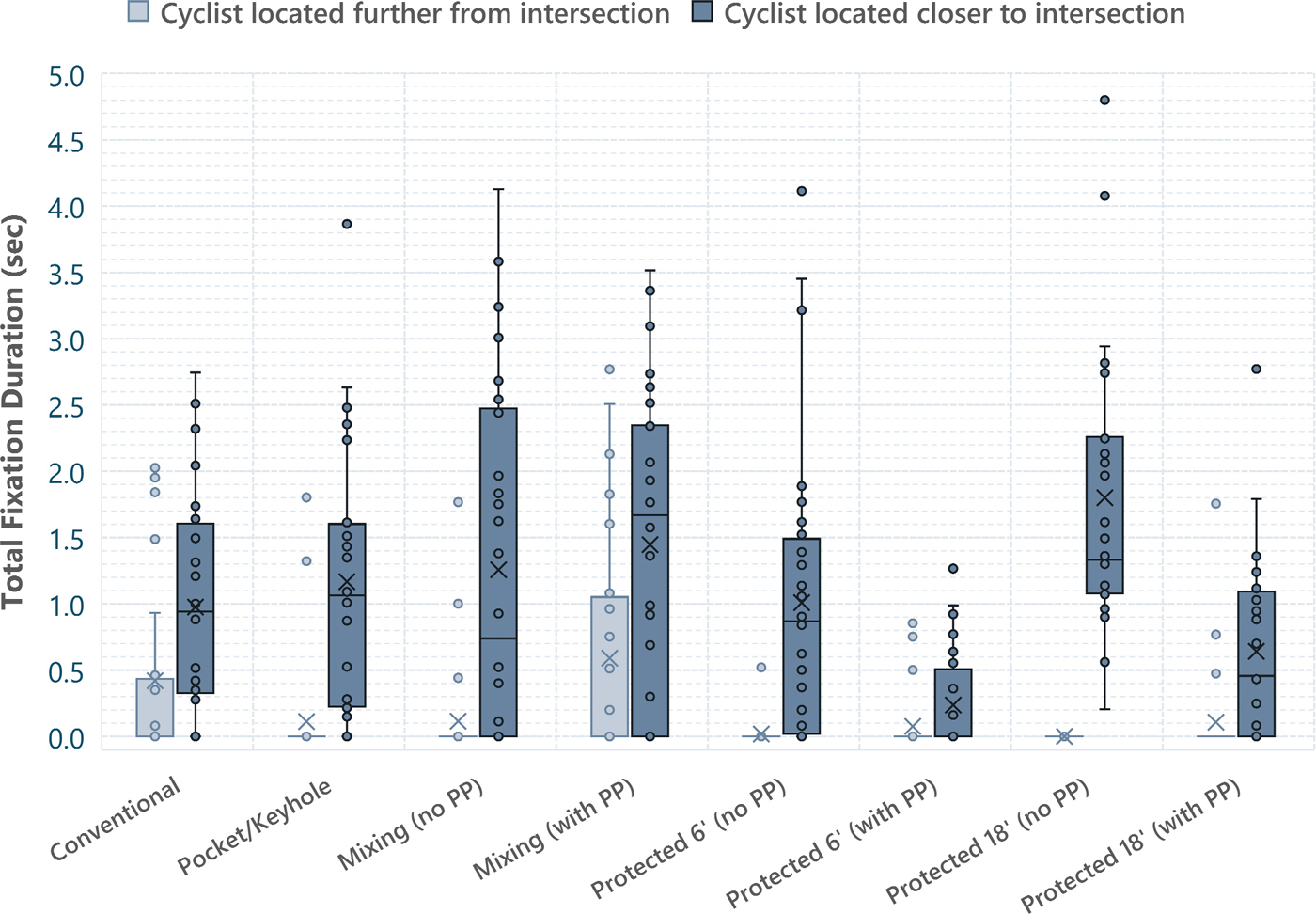
Table 82. Descriptive Statistics of the Distribution of TFD on Cyclists by Scenario
| Convent. Bike Lane | Pocket/Key hole | Mixing (no PP) | Mixing (w. PP) | Protected 6' (no PP) | Protected 6' (w. PP) | Protected 18' (no PP) | Protected 18' (w. PP) | |||||||||
|---|---|---|---|---|---|---|---|---|---|---|---|---|---|---|---|---|
| Far | Near | Far | Near | Far | Near | Far | Near | Far | Near | Far | Near | Far | Near | Far | Near | |
| Avg | 0.42 | 0.98 | 0.11 | 1.17 | 0.11 | 1.26 | 0.59 | 1.45 | 0.02 | 1.01 | 0.08 | 0.24 | 0 | 1.80 | 0.11 | 0.64 |
| Med | 0 | 0.94 | 0 | 1.06 | 0 | 0.74 | 0 | 1.67 | 0 | 0.87 | 0 | 0 | 0 | 1.33 | 0 | 0.46 |
| Stdv | 0.71 | 0.82 | 0.41 | 1.00 | 0.38 | 1.33 | 0.91 | 1.18 | 0.10 | 1.10 | 0.23 | 0.40 | 0 | 1.12 | 0.36 | 0.70 |
When the cyclist is located closer to the intersection, participants spent more time fixating on the cyclist. Across all intersections, the average time a participant spent looking at a cyclist (from the approach to turn zone) was 1.07 seconds (SD = 0.48 sec). The maximum average TFD, 1.80 seconds, was observed in the protected intersection (offset by 18’, and no parallel parking). Whereas the minimum average TFD, 0.24 seconds, was observed in the protected intersection (offset by 6’, with parallel parking). Macroscopically, these trends may translate to the scenario-level, but the statistical values do not account for the difference in roadway geometry, zone lengths and location of conflict points. Hence, this data is assessed at a smaller granularity, by the four intersection designs (conventional, keyhole, mixing zone, protected). Similarities between varying intersection designs are introduced, calling attention to the contrast between geometric designs and visual attention.
As visualized in Figure 42 and detailed in Table 82, the characteristics of the distributions at intersections with the conventional and pocket/keyhole bike lanes was notably similar, where the average TFD at the conventional bike lane scenarios was 0.98 seconds (SD = 0.82 sec.) and that of the pocket/keyhole scenarios was 1.17 seconds (SD = 1.00 sec).
For the mixing zone scenarios, participants looked at the cyclist for similar durations ( = 1.35 sec), regardless of parallel parking levels. When parallel parking was not present, the average fixation duration on cyclists was 1.26 sec. (SD = 1.30 sec) and slightly higher when parallel parking was present, with an average of 1.45 seconds (SD = 1.18 sec). Moreover, these distributions are relatively similar with and without parallel parking. Whereas at protected intersections, at both offsets, participants visually attended to cyclists for longer durations with greater variance when parallel parking was not present.
When the cyclist was located further from the intersection, drivers spent less time looking at the cyclist. Across most intersections, the third and first quartiles had values of zero and correspondingly low means. However, this was not the case for two scenarios: conventional and mixing zone (with parallel parking). At these scenarios, drivers spent a notably higher amount of time looking at the cyclists, with the highest being 0.59 seconds, observed at the mixing zone (with parallel parking) scenario (SD = 0.91 sec) and the other being 0.42 seconds, observed at the conventional scenario (SD = 0.71 sec).
AOI: Pavement Markings
In Figure 43, the distributions of the participants’ time spent looking at pavement markings (from the start of the approach zone to the end of the turn zone) is shown by scenario, and further distinguished by the relative location of the cyclist. Following this plot, Table 83 organizes the descriptive statistics corresponding to the boxplots.
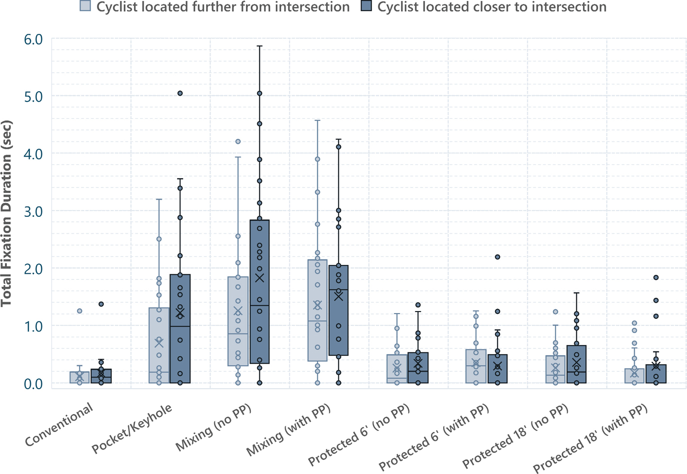
Table 83. Descriptive Statistics of the Distribution of TFD on Pavement Markings by Scenario
| Convent. Bike Lane | Pocket/Keyhole | Mixing (no PP) | Mixing (w. PP) | Protected 6' (no PP) | Protected 6' (w. PP) | Protected 18' (no PP) | Protected 18' (w. PP) | |||||||||
|---|---|---|---|---|---|---|---|---|---|---|---|---|---|---|---|---|
| Far | Near | Far | Near | Far | Near | Far | Near | Far | Near | Far | Near | Far | Near | Far | Near | |
| Avg | 0.11 | 0.17 | 0.30 | 0.68 | 1.25 | 1.83 | 1.35 | 1.50 | 0.26 | 0.34 | 0.35 | 0.29 | 0.26 | 0.36 | 0.17 | 0.29 |
| Med | 0 | 0.10 | 0 | 0.18 | 0.85 | 1.35 | 1.08 | 1.62 | 0.08 | 0.20 | 0.30 | 0 | 0.13 | 0.19 | 0 | 0 |
| Stdv | 0.24 | 0.27 | 0.49 | 1.09 | 1.25 | 1.66 | 1.22 | 1.19 | 0.33 | 0.39 | 0.39 | 0.50 | 0.33 | 0.45 | 0.30 | 0.50 |
Given the lateral shifting of the vehicle travel lanes, and subsequently the ROW, at the pocket/keyhole bike lane and mixing zone intersections, there existed more pavement markings when compared to the protected intersection and conventional bike lane. This was reflected in the visual attention data as the average TFD on pavement markings at the pocket/keyhole bike lane and mixing zone intersections was 1.22 seconds higher than that of the protected intersection and conventional bike lane when the cyclist was located closer to the intersection.
- Pocket/Keyhole, Mixing Zone (no PP), Mixing Zone (with PP) = 1.52 seconds.
- Conventional Bike Lane, Protected Intersections (both offsets and parallel parking levels = 0.29 seconds.
The greatest average TFD was observed at the mixing zone intersection, without parallel parking, when the cyclist was located closer to the intersection (Near = 1.83 seconds, SD = 1.66 seconds). At the same cyclist location level, the minimum average TFD was observed at the conventional bike lane (Near = 0.17 seconds, SD = 0.27 seconds).
At an intersection-level basis, the TFD on pavement markings was not expected to vary greatly by cyclist location level. There is a slight observable increase in average TFD when the cyclist is located closer to the intersection and may be explained by increased exposure times due to decreased speeds.
AOI: Parallel Parking
In Figure 44, the distributions of the participants time spent looking at the parallel parking (from the start of the approach zone to the end of the turn zone) is shown by scenario, further distinguished by the relative location of the cyclist. Following this plot, the corresponding descriptive statistics are organized in Table 84.
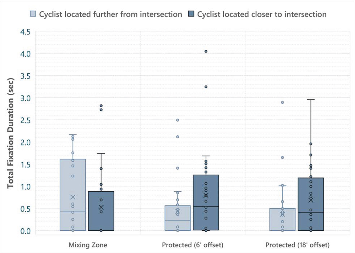
Table 84. Descriptive Statistics of the Distribution of TFD on Parallel Parking by Scenario
| Mixing Zone (with PP) | Protected 6' (with PP) | Protected 18' (with PP) | ||||
|---|---|---|---|---|---|---|
| Far | Near | Far | Near | Far | Near | |
| Avg | 0.75 | 0.52 | 0.44 | 0.79 | 0.36 | 0.68 |
| Med | 0.42 | 0 | 0.23 | 0.54 | 0 | 0.41 |
| Stdv | 0.80 | 0.82 | 0.64 | 0.98 | 0.65 | 0.79 |
The parallel parking, by design and nature, obstructs the visibility of cyclists who are near the intersection. Moreover, parallel parking disrupts the ability for drivers to maintain their visual attention on the cyclist, implying less precision and potential for more error with determining the relative proximity of the cyclist. In an attempt to keep tracking the cyclist behind the parallel parking, multiple drivers exhibited visual attention on the parallel parking while doing so. Unlike the mixing zone intersections, at the intersections with protected bike lanes, participants’ visual attention on the parallel parked cars were higher when the cyclist was located closer to the intersection. The average TFD on parallel parking was relatively similar between the two bike lane offsets, being 0.74 seconds (cyclist=near) and 0.40 seconds (cyclist=far).
For the mixing zone intersections, TFDs were higher when the cyclist was further from the intersection (Near = 0.52 seconds vs. far = 0.75 seconds). This difference in relationship may be explained by the proximity
of the parallel parking to the conflict point – at the mixing zone intersections, there is less distance between the conflict point and the last parallel parked car. Thus, visually locating the cyclist may be more important as the driver is passing the parallel parking, warranting more visual attention on where the cyclist would be (behind the parallel parked cars) and instead be observed as TFD on the parallel parking.
AOI: Mirrors (Rear-and right side-view)
Figure 45 shows the distribution of the cumulative time a participant spent looking at their rear-view and right side-view mirrors (from the start of the approach zone to the end of the turn zone)6. The corresponding descriptive statistics are organized in Table 85.
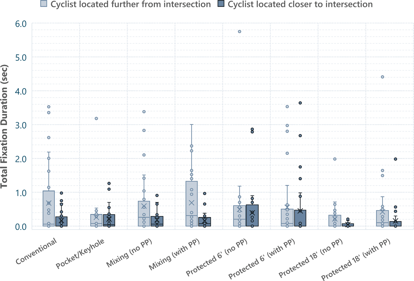
___________________
6 One outlier was removed to optimize the utility of the plot area and improve the readability of the box and whisker plots. The outlier was observed in the Separated Bike Lane (no parallel parking, 6′ offset) scenario, with an average TFD of 5.8 seconds.
Table 85. Descriptive Statistics of the Distribution of TFD on Mirrors by Scenario
| Conventional Bike Lane | Pocket/Keyhole | Mixing (no PP) | Mixing (w. PP) | Protected 6' (no PP) | Protected 6' (w. PP) | Protected 18' (no PP) | Protected 18' (w. PP) | |||||||||
|---|---|---|---|---|---|---|---|---|---|---|---|---|---|---|---|---|
| Far | Near | Far | Near | Far | Near | Far | Near | Far | Near | Far | Near | Far | Near | Far | Near | |
| Avg | 0.68 | 0.17 | 0.26 | 0.21 | 0.59 | 0.18 | 0.69 | 0.16 | 0.49 | 0.40 | 0.56 | 0.45 | 0.21 | 0.04 | 0.42 | 0.15 |
| Med | 0.06 | 0 | 0.08 | 0.04 | 0.26 | 0.06 | 0.31 | 0.07 | 0.20 | 0 | 0.08 | 0 | 0 | 0 | 0.10 | 0 |
| Stdv | 1.08 | 0.28 | 0.60 | 0.33 | 0.89 | 0.28 | 0.85 | 0.23 | 1.08 | 0.75 | 1.01 | 0.90 | 0.41 | 0.08 | 0.89 | 0.39 |
Overall, and as expected, drivers spent more time looking at their rear-view and right side-view mirrors when the cyclist was located further from the intersection (t=0.49 seconds) as opposed to when the cyclist was located closer to the intersection (t=0.22 seconds). When the cyclist was located further from the intersection, the maximum averages were observed at mixing zone (no PP) and conventional scenarios, with averages of 0.69 seconds and 0.68 seconds, respectively. When cyclists were located closer to the intersection, the maximum average TFDs were observed at the protected (6’ offset) scenarios – 0.45 seconds when parallel parking was present and 0.40 seconds when parallel parking was not present.
There was expected to be an observable decrease in TFD when the cyclists were located closer to the intersection. This was not the case for the keyhole, and 6’-offset protected intersections (no PP and with PP) scenarios, as the average difference in TFDs between cyclist location levels was 0.08 seconds. Whereas, for the other 13 scenarios, this average difference was 0.38 seconds. Consistent across all scenarios, is the observable increase in spread in TFDs when the cyclists are located further from the intersection.
Speed
The vehicle speed data was measured and collected via SimObserver. The average vehicle speeds are presented for general observations and comparisons. Following, the minimum vehicle speeds, only of near cyclist location scenarios, are presented, as these are indicative of driver yielding behavior. A single plot presenting all data at this level would constrain the ability to observe and reference the descriptive statistics and trends. Hence, the data is further subdivided into individual plots by location of the cyclist.
Average Speeds
Cyclist Located Closer to Intersection
In Figure 46, the distribution of average speeds per zone are presented by scenario. The corresponding descriptive statistics are organized in Table 86.
Table 86. Descriptive Statistics of Average Speeds per Zone by Scenario (Cyclist = Near)
| Convent. Bike Lane | Pocket/keyhole | Mixing (no PP) | Mixing (w. PP) | Protected 6' (no PP) | Protected 6' (w. PP) | Protected 18' (no PP) | Protected 18' (w PP) | ||
|---|---|---|---|---|---|---|---|---|---|
| Approach | 17.4 | 18.4 | 19.3 | 19.0 | 20.3 | 21.3 | 20.0 | 20.8 | |
| ⊽ | Transition | 13.3 | 14.0 | 10.2 | 11.1 | 14.6 | 16.8 | 13.1 | 14.3 |
| Turn | 9.8 | 11.5 | 11.3 | 11.5 | 8.7 | 10.3 | 9.3 | 10.1 | |
| Approach | 16.6 | 17.3 | 17.9 | 17.9 | 20.0 | 22.1 | 20.0 | 20.8 | |
| ṽ | Transition | 11.9 | 12.4 | 6.9 | 10.2 | 12.1 | 16.8 | 12.5 | 13.4 |
| Turn | 8.7 | 10.1 | 9.9 | 10.5 | 7.4 | 10.7 | 9.3 | 9.8 | |
| Approach | 4.7 | 4.6 | 5.0 | 4.6 | 4.7 | 4.4 | 2.9 | 3.7 | |
| σ | Transition | 4.4 | 5.7 | 7.1 | 5.1 | 6.1 | 4.8 | 3.0 | 4.7 |
| Turn | 3.6 | 3.9 | 3.5 | 3.1 | 3.0 | 5.0 | 1.3 | 2.5 |
The average speed by zone was 19.9 mph (SD = 0.87 mph) for the approach zone, 13.4 mph (SD = 2.11 mph) for the transition zone, and 10.3 mph (SD = 1.04 mph) for the turn zone. While these may macroscopically depict trends at a scenario-level, these statistical values do not account for the difference in roadway geometry, zone lengths, and location of conflict points. Hence, this data is assessed at a smaller granularity, by the four intersection designs (conventional, keyhole, mixing zone, protected). Similarities between varying intersection designs are introduced, calling attention to the contrast between geometric designs and vehicle speeds.
All scenarios, except the mixing zone scenarios, exhibited the expected pattern in a consistent decrease in speeds from the approach to turn zone. In the mixing zone scenarios, the average and median speeds were lowest in the transition zone, with average and median speeds being higher in the turn zone. It should be noted that due to the geometric design of the mixing zone, the vehicle-bicycle conflict point is in the transition zone, which otherwise is in the turn zone for all other scenarios.
Looking at the mixing zone intersection, the average speeds exhibited small differences across parallel parking levels. The average speeds for each zone are as follows: approach zone: 19.2 mph (SD = 0.16 mph), transition zone: 10.6 mph (SD = 0.57 mph) and turn zone: 11.4 mph (SD = 0.09 mph). Unlike all other scenarios, an increase in average speeds from the transition to turn zone was observed (no PP: ΔvTrans.→Turn = + 1.1 mph; with PP: ΔvTrans.→Turn = + 0.4 mph). For the mixing zone scenarios, the average speeds were expected to be lowest in the transition zone as it contains the vehicle-bicycle conflict point. In the next subsection, the minimum speeds per zone and scenario, this relationship is observable.
Regarding the transition zone, for the protected intersections, the distribution of average speeds was greater when the offset was 6 feet (SDoffset=6’ = 5.45 mph; SDoffset=18’ = 3.85 mph). More interestingly, for these intersections, the average speeds of the transition zones increased when parallel parking was present (Δ voffset=6’ = + 2.3 mPh; Δ voffset=18’ = + 1.2 mph).
In Table 87, the effect of parallel parking on speeds by zone are shown, where the values are the average change in speeds from the no parallel parking scenario to its corresponding parallel parking present scenario. Regarding the protected intersections, the average speeds in each zone were slightly less when parallel parking was present. For the 6’-offset scenarios only, when parallel parking was present, the average speeds for the approach, transition and turn zone were 1.1, 2.3 and 1.6 mph lower than the corresponding speeds when there was no parallel parking. Similarly, this was exhibited when the offset was 18’. When parallel parking was present, the average speeds for the approach, transition and turn zone were 0.7, 1.2 and 0.8 mph lower than the corresponding speeds when there was no parallel parking.
| Mixing Zone | Protected (6' offset) | Protected (18' offset) | |
|---|---|---|---|
| Approach | -0.2 | 1.1 | 0.7 |
| Median | 0.8 | 2.3 | 1.2 |
| Std. Deviation | 0.1 | 1.6 | 0.8 |
Cyclist Located Further from Intersection
In Figure 47, the distribution of average speeds per zone are presented by scenario. The corresponding descriptive statistics are organized in Table 88.
Table 88. Descriptive Statistics of Average Speeds per Zone by Scenario (Cyclist = Far)
| Convent. Bike Lane | Pocket/Keyhole | Mixing (no PP) | Mixing (w. PP) | Protected 6' (no PP) | Protected 6' (w. PP) | Protected 18' (no PP) | Protected 18' (w PP) | ||
|---|---|---|---|---|---|---|---|---|---|
| ⊽ | Approach | 19.9 | 21.6 | 22.9 | 19.5 | 24.5 | 23.2 | 23.8 | 22.6 |
| Transition | 16.2 | 18.1 | 17.7 | 11.9 | 20.1 | 18.4 | 19.2 | 17.4 | |
| Turn | 10.6 | 13.6 | 14.4 | 11.7 | 11.7 | 11.1 | 12.7 | 11.7 | |
| ṽ | Approach | 20.4 | 22.1 | 24.1 | 19.2 | 24.9 | 23.4 | 23.8 | 23.6 |
| Transition | 16.0 | 18.9 | 19.4 | 11.5 | 19.9 | 18.5 | 19.0 | 17.6 | |
| Turn | 9.8 | 13.6 | 14.9 | 11.4 | 11.5 | 11.4 | 12.8 | 12.1 | |
| σ | Approach | 5.4 | 4.2 | 4.3 | 5.2 | 3.7 | 3.5 | 3.0 | 4.3 |
| Transition | 5.5 | 4.4 | 6.5 | 6.5 | 4.1 | 3.9 | 3.9 | 4.5 | |
| Turn | 5.0 | 2.9 | 3.2 | 2.9 | 2.4 | 3.3 | 2.7 | 3.2 |
Overall, the average speed by zone was 22.6 mph (σ = 1.64 mph) for the approach zone, 17.4 mph (σ = 2.45 mph) for the transition zone, and 12.2 mph (SD = 1.28 mph) for the turn zone. While these may macroscopically depict trends at a scenario-level, these statistical values do not account for the difference in roadway geometry, zone lengths and location of conflict points. Hence, this data are assessed at a smaller granularity, by the four intersection designs (conventional, keyhole, mixing zone, protected). Any similarities between different intersection designs are introduced with the reminder of difference in lengths and roadway design in each zone.
For the protected intersections, the distributions and differences between two consecutive zones was similar between scenarios. For all four scenarios, the average speeds in the approach zone, transition zone and turn zone were 23.5 mph, 18.8 mph and 11.8 mph, respectively.
For the mixing zone intersection, there existed more variance in the average speeds between the two scenarios. When parallel parking was not present, average speeds were higher in each zone. In the approach zone, the average speeds across both scenarios exhibited the least difference (νno PP = 22.9, νwith PP = 19.5 mph). However, in the transition zone, the average speed in the scenario with parallel parking, was 5.8 mph lower than the average speed of the no parallel parking scenario (vno PP = 17.7, vwith PP = 11.9 mph). Similarly but at a smaller magnitude, this relationship was exhibited in the transition zone (Δv = 2.7, vno PP = 14.4, vwith PP = 11.7 mph).
In Table 89, the effect of parallel parking on speeds by zone are shown, where the values are the average change in speeds from the no parallel parking scenario to its corresponding parallel parking present scenario.
| Mixing Zone | Protected (6' offset) | Protected (18' offset) | |
|---|---|---|---|
| Approach | 0.11 | 0.17 | 0.30 |
| Median | 0 | 0.10 | 0 |
| Std. Deviation | 0.24 | 0.27 | 0.49 |
Regarding the protected intersections, the average speeds in each zone were slightly less when parallel parking was present. For the 6’-offset scenarios only, when parallel parking was present, the average speeds for the approach, transition and turn zone were 1.2, 1.7 and 0.5 mph lower than the corresponding speeds when there was no parallel parking. Similarly, this was exhibited when the offset was 18’. When parallel parking was present, the average speeds for the approach, transition and turn zone were 1.1, 1.8 and 0.9 mph lower than the corresponding speeds when there was no parallel parking.
When compared to the protected intersections, the presence of parallel parking had a greater influence on average zone speeds for the mixing zone intersection. When parallel parking was introduced, the average speeds decreased by 3.2 mph in the approach zone, 5.6 mph in the transition zone and 2.6 mph in the turn zone.
Interestingly, the average speeds in the pocket/keyhole scenario were most like that of the mixing zone (no PP) intersection. In comparison to the mixing zone (no PP), the average speeds in the approach and turn zone of the pocket/keyhole intersection were 1.2 and 0.8 mph higher, respectively. Whereas for the transition zone, the average speed in the pocket/keyhole intersection was 0.4 mph lower than that of the mixing zone (no PP). It should be noted that the starting and ending points of the zones are different between
these intersections. Moreover, the corresponding geometric designs at and within these boundaries are different. However, in the pocket/keyhole and mixing zone intersections, their geometry is designed such that the conflict point is located at a distance upstream of the stop bar, as opposed to the intersections with conventional and protected intersections.
Minimum Speeds
A participant’s yielding behavior towards the cyclist can be captured by looking at the absolute minimum speed driven in the zones closest to the conflict point. This subsection presents the distribution of minimum speeds that drivers decelerated to. Like the average speed observations, the data is presented at a per-zone level by scenario, by zone type. Considering the implications of minimum speeds, the approach zone was intentionally removed as its minimum speeds do not pose the same implications as that of the downstream zones. It should be noted that unlike the average speed observations, these data points do not generalize drivers’ behaviors across the entire zone as the minimum speed represents the driver behavior at a single point in time.
Cyclist Located Closer to Intersection
In Figure 48, the distribution of average speeds per zone are presented by scenario. The corresponding descriptive statistics are organized in Table 90.
| Convent. Bike Lane | Pocket/Keyhole | Mixing (no PP) | Mixing (w. PP) | Protected 6' (no PP) | Protected 6' (w. PP) | Protected 18' (no PP) | Protected 18' (w PP) | ||
|---|---|---|---|---|---|---|---|---|---|
| ⊽ | Transition | 10.6 | 11.8 | 7.5 | 9.1 | 11.6 | 14.1 | 10.3 | 11.0 |
| Turn | 6.5 | 8.4 | 8.6 | 8.9 | 5.5 | 5.2 | 6.3 | 6.8 | |
| ṽ | Transition | 9.5 | 10.8 | 4.9 | 7.7 | 8.7 | 14.1 | 10.1 | 9.7 |
| Turn | 6.3 | 7.8 | 7.7 | 8.5 | 5.3 | 5.6 | 6.9 | 6.6 | |
| σ | Transition | 4.5 | 6.3 | 8.0 | 5.7 | 6.4 | 5.2 | 2.8 | 5.5 |
| Turn | 4.0 | 4.8 | 4.1 | 3.8 | 3.0 | 4.5 | 3.2 | 3.8 |
Considering the cyclist was located closer to the intersection, the minimum speeds are indicative of drivers’ yielding behaviors. Moreover, because of the relative proximity of the cyclist, it was expected for larger spreads to occur within a scenario and for there to be less uniformity across scenarios. This is observed visually in Figure 48, with a range in averaged minimum speeds of 6.6 mph for the transition zone and 3.7 mph for the turn zone. Across all scenarios, the lowest averaged minimum speed exhibited in the transition zone was observed in the Mixing Zone (no parallel parking) as 7.5 mph (SD = 8.06 mph). Likewise, for the turn zone, the lowest averaged minimum speed was observed in the protected intersection (with parallel parking, 6’ offset) scenario as 5.2 mph (SD = 4.52 mph).
The average minimum speeds for the mixing zone can be assessed exclusively, given the conflict point is shifted upstream to the transition zone. In this zone, their averaged minimum speed equates to 8.3 mph. As expected, the averaged minimum speed in the turn zone was slightly higher at 8.75 mph.
Regarding the intersection with a pocket/keyhole bike lane, the transition and turn zone, the average minimum speeds were 11.8 mph (SD = 6.34 mph) and 8.4 mph (SD = 4.84 mph), respectively. The averages and distributions of the turn zone minimum speeds were most like those of the mixing zone intersections. With reference to the standard deviations observed at the mixing zone intersections, that of the pocket/keyhole is relatively higher at 4.84. Like the mixing zone, the conflict point is shifted upstream of the intersection. However, the conflict “point” is best described as a region, as there is a longitudinal distance over which the driver can come in conflict with the adjacent cyclist.
For the protected intersections and the conventional bike lane, the minimum speed in the turn zone is most indicative of turning behavior as the conflict point is at the intersection. For the conventional scenario, the average minimum speed observed in the transition zone and turn zone were 10.6 mph (SD = 4.52 mph) and 6.5 mph (SD = 4.03 mph), respectively.
Cyclist Located Further from Intersection
In Figure 49 distribution of average speeds per zone are presented by scenario. The corresponding descriptive statistics are organized in Table 91.
| Convent. Bike Lane | Pocket/Keyhole | Mixing (no PP) | Mixing (w. PP) | Protected 6' (no PP) | Protected 6' (w. PP) | Protected 18' (no PP) | Protected 18' (w PP) | ||
|---|---|---|---|---|---|---|---|---|---|
| ⊽ | Transition | 13.2 | 16.5 | 15.9 | 9.3 | 17.3 | 15.8 | 16.9 | 14.9 |
| Turn | 7.3 | 11.7 | 11.9 | 9.1 | 9.1 | 8.5 | 10.5 | 9.3 | |
| ṽ | Transition | 12.4 | 16.9 | 17.8 | 8.8 | 17.1 | 16.2 | 17.4 | 15.8 |
| Turn | 7.3 | 11.5 | 12.9 | 8.9 | 9.0 | 9.7 | 11.3 | 10.3 | |
| σ | Transition | 6.2 | 4.7 | 7.0 | 7.6 | 4.2 | 4.3 | 4.4 | 5.1 |
| Turn | 6.4 | 3.1 | 3.3 | 3.6 | 2.6 | 4.0 | 3.5 | 4.2 |
GSR
The GSR data were measured and recorded using the Shimmer3 GSR+, which was paired with the iMotions software for reduction. The GSR data is presented as average PPM to control the natural variation between participants’ peak measures. The magnitude represents participants’ reactions, in terms of level of stress, to the scenarios.
In Figure 50, the distribution of maximum PPM (per zone) are presented by scenario. The corresponding descriptive statistics are organized in Table 92.
Of all intersection designs, the pocket/keyhole intersection exhibited the greatest GSR peaks for both cyclist location levels. Interestingly, when cyclists were located further from the intersection, GSR peaks increased. Moreover, the corresponding spreads were larger. These large spreads were also observed in scenarios when the cyclist was located closer to the intersection. However, this was not the case for mixing zones, as their spreads were tighter. Looking at all scenarios, the pocket/keyhole bike lane and both mixing zone intersections exhibited observably higher 1st quartile values at both levels of the cyclist location variable. This observation was reflected in participants’ level of stress when maneuvering through the protected bike lane configuration (6’ offset, no PP) with the cyclist located closer to the intersection. In comparison to the three other protected bike lane configurations, and when the cyclist was located closer to the intersection, this configuration was the only one with a 25th percentile greater than zero.
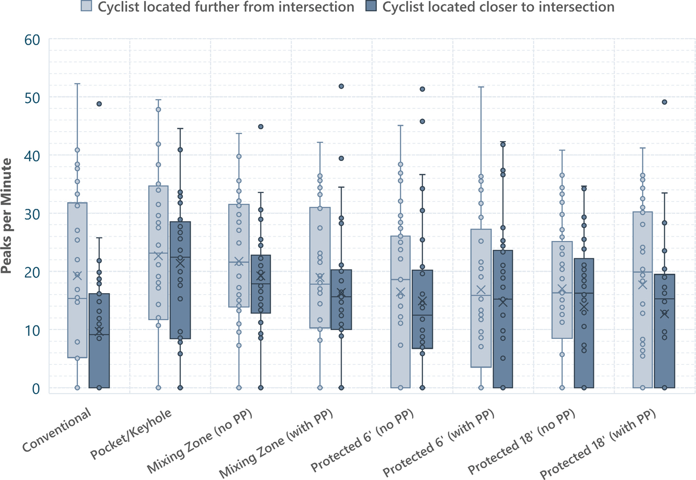
Table 92. Descriptive Statistics of Distribution of Maximum PPM Across All Zones by Scenario
| Convent. Bike Lane | Pocket/Keyhole | Mixing (no PP) | Mixing (w. PP) | Protected 6' (no PP) | Protected 6' (w. PP) | Protected 18' (no PP) | Protected 18' (w. PP) | |||||||||
|---|---|---|---|---|---|---|---|---|---|---|---|---|---|---|---|---|
| Far | Near | Far | Near | Far | Near | Far | Near | Far | Near | Far | Near | Far | Near | Far | Near | |
| Mean [–PPM] | 19.2 | 9.7 | 22.7 | 21.4 | 21.7 | 19.2 | 19 | 16.4 | 16.5 | 14.9 | 16.8 | 14.7 | 17 | 13.9 | 17.7 | 12.7 |
| Median [(PPM)~] | 15.3 | 9.1 | 23.1 | 22.4 | 21.6 | 17.9 | 17.8 | 15.6 | 18.6 | 12.5 | 15.9 | 15.2 | 16.3 | 16.2 | 19.9 | 15.3 |
| Std. Dev. [a] | 19.2 | 10.2 | 15.3 | 18.4 | 11.8 | 14 | 12.6 | 11.3 | 13.4 | 12.8 | 13.3 | 13.4 | 12 | 11.1 | 13.6 | 11.6 |
Speed Profiles and Visual Attention
To provide more insight into the relationship between drivers’ speed and visual attention throughout the intersection approach and turning movement, participant-level visual attention data on the cyclist and their corresponding speed data was plotted against vehicle position. In Figure 51, participant-level data from each of the eight bike lane configurations is depicted. These plots were generated only for the near cyclist condition, as the implications of driver’s visual attention and speed are of greatest interest.
For an intersection, the diagram contains two plots, with the top-most plot showing the distribution of the visual attention (seconds) on the cyclist per data collection zone – each diagram has the same vertical axis bounds, 0 to 2.5 seconds. The line plot below illustrates the vehicle speed (mph) versus position in feet from the end of the turn zone – each plot has the same vertical axis bounds, 0 to 35 mph. All plots have the same horizontal axis bounds of 0 to 200 feet, except for the mixing zone intersection, which extend to 210 feet, as the start of their approach zone was 210 feet setback from the turn. Individual speed profiles are represented by the light blue lines, whereas the averaged speed profile is depicted by the thicker, dark blue line. This speed profile was generated by averaging the speeds across participants at each unit distance. Aerial images of the corresponding vehicle-bicycle lane configurations are located directly below the speed plot and are aligned such that the horizontal axes line up with the corresponding regions of data collection.
It is important to note that the full participant sample is not depicted in the following plots. For data to be included in a scenario’s plot, a participant’s corresponding speed and visual attention datasets could not have been lost or incomplete due to equipment malfunctions. As mentioned in Table 79, 12 participants’ eye tracking data and two different participants’ speed data were not recorded, hence the maximum available subsample size for a scenario was reduced by 14 participants to n=26. Recall that data was recorded on a per scenario basis. There were instances where participants had an incomplete speed or eye tracking dataset for a single scenario, likely due to a brief disconnection in the equipment while they were executing that drive. These were unpredictable and occurred randomly among participants. If this occurred in either the speed or eye tracking dataset for a participant, their dataset was excluded and not plotted for the corresponding scenario. Consequently, this further reduced the plotted sample size by scenario. These adjusted sample sizes varied by scenario and are denoted at the top left of each plot.
Post-Drive Survey
Level of Familiarity
Table 93 shows the reported level of familiarity with intersections. Most participants were familiar with conventional bike lane (100%) and pocket/keyhole bike lane (67.5%). Participants were least familiar with the mixing zone intersection (85%) and protected intersection (67.5%).
Table 93. Reported Level of Familiarity with Intersections
| Question | Bike Lane Configuration | Response | Count | Percentage |
|---|---|---|---|---|
| Prior to this experiment, what best describes your familiarity with a [bike lane/intersection type] as shown in the images below? | Conventional Bike Lane | Familiar | 40 | 100.0% |
| Partially familiar | 0 | 0.0% | ||
| Unfamiliar | 0 | 0.0% | ||
| Pocket/Keyhole Bike Lane | Familiar | 27 | 67.5% | |
| Partially familiar | 6 | 15.0% | ||
| Unfamiliar | 7 | 17.5% | ||
| Mixing Zone | Familiar | 6 | 15.0% | |
| Partially familiar | 10 | 25.0% | ||
| Unfamiliar | 24 | 60.0% | ||
| Protected Intersection | Familiar | 13 | 32.5% | |
| Partially familiar | 12 | 30.0% | ||
| Unfamiliar | 15 | 37.5% |
Level of Comfort
Levels of comfort when cyclists were present was greatest for the conventional bike lane (average = 69.4) and pocket/keyhole bike lane (average = 56.5) and lowest for the mixing zone scenarios (average = 47.2) and protected intersection scenarios (average = 50.6) Table 94 presents these findings.
Levels of comfort when cyclists were not present was greatest for the conventional bike lane (average = 94.5) and was similar between the pocket/keyhole (average = 84.9) and protected intersection scenarios (average = 83.3), with the mixing zone having the lowest reported level of comfort (average = 78.7).
Question: For the [intersection/bike lane type], what was your level of comfort when navigating each of the intersections when a cyclist was present in the bike lane versus when a cyclist was not present in the bike lane? (0 = no comfort, highly stressful, 100 = maximum comfort, not stressful)
Table 94. Level of Comfort by Presence of Cyclist per Intersection
| Conventional Bike Lane | Pocket/Keyhole | Mixing Zone | Protected Intersection | |||||
|---|---|---|---|---|---|---|---|---|
| Cyclist Present | No Cyclist Present | Cyclist Present | No Cyclist Present | Cyclist Present | No Cyclist Present | Cyclist Present | No Cyclist Present | |
| Mean | 69.4 | 94.5 | 56.5 | 84.9 | 47.2 | 78.7 | 50.6 | 83.3 |
| Median | 71.0 | 100.0 | 55.0 | 91.5 | 46.5 | 85.0 | 47.0 | 90.0 |
| Std. Dev. | 23.5 | 11.0 | 26.0 | 18.1 | 26.1 | 20.3 | 26.0 | 22.4 |
Parallel Parking and Cyclist Visibility
Most participants reported parallel parking to have affected their ability to see cyclists in the mixing zone (80%) and protected intersection scenarios (87.5%) (Table 95).
Table 95. Reported Effect of Parallel Parking on Visibility of Cyclist
| Question | Bike Lane Configuration | Response | Count | Percentage |
|---|---|---|---|---|
| Did the presence of parallel parking affect your ability to see any of the cyclists (with respect to stated intersection type)? | Mixing Zone Intersection | Yes | 32 | 80.0% |
| No | 6 | 15.0% | ||
| I do not remember | 2 | 5.0% | ||
| Protected Intersection | Yes | 35 | 87.5% | |
| No | 5 | 12.5% | ||
| I do not remember | 0 | 0.0% |
Human Factors Study Summary
In the following section, the most insightful findings and observations with potential implications on driver and cyclist safety are discussed. Given the quantity of results and scope of the project, unless explicitly stated, all intersections in the discussion refer only to the results of the scenario where the cyclist was located closer to the intersection, and therefore, does not necessarily apply to both levels of cyclist proximity.
Visual Attention
Across the conventional bike lane, pocket/keyhole, and protected 6’ offset bike lane (no parallel parking), drivers exhibited similar visual attention on the cyclist. This similarity is not unexpected as each of their bicycle lane configuration designs yield unobstructed visibility of the cyclist throughout the entire intersection approach. Like these intersection designs, the protected 18’ offset bike lane intersection (no PP) did not obstruct the cyclist visibility. However, at this intersection, a significantly greater percentage of drivers looked at the cyclist and when they did, their fixation times were longer. Moreover, this was the
only intersection design where all participants had a non-zero fixation time on the cyclist. Given the 18’ offset bike lane, cyclists had to traverse a longer distance to reach the point of crossing, resulting in longer durations of exposure. Another rationale for the higher fixation times may be due to drivers trying to comprehend and predict the cyclist’s trajectory and accurately gauge their speed. The geometric design of the bike lane configuration has cyclists travel diagonally away from the vehicle trajectory to reach the offset crossing – this atypical, diverging trajectory may be harder for drivers to discern, and hence, be an attraction for more visual attention on the cyclist, and subsequently impose an increased workload on the driver. Further, the change in direction of the cyclist, from what was previously parallel to the driver’s trajectory, warrants a change in how drivers gauge the cyclist’s speed and relative proximity.
Inherent to design, decreased visual attention on the cyclists were observed upon the inclusion of parallel parking at protected intersections. Whereas at the mixing zone intersections, drivers’ visual attention on the cyclist was consistent across parallel parking conditions. This would be expected if the bicycle lane was instead between the vehicle travel lane and parallel parking; however, this is not the case as the presence of parallel parking reduces the duration of time and length of travel distance that the cyclist is within direct line of sight when at or downstream of the positioning of the vehicle. Implying that the visual attention on cyclists in this scenario could have only occurred between the downstream end of the parallel parked cars and the turning maneuver, these values likely correspond to increased yielding behaviors among drivers. This was corroborated through using the participant-level speed profile and visual attention data – participants who exhibited higher fixation duration on the cyclist in the transition zone (from beginning of turn bay to yield triangles) correspond to the participants whose speed profiles exhibited local minimums less than 5 mph on the speed profile plots. Moreover, similar visual attention behaviors were exhibited in the turn zone; for drivers to fixate on the cyclist, they would need to be following behind the cyclist, implying drivers yielding towards cyclists.
Overall, the TFD values were observed to be greater when the cyclist was closer to the intersection. In part, this finding is a result of the experimental design – in the scenarios where the cyclist was located further from the intersection, a majority of the drivers passed the cyclist upstream of the data collection zones, and hence, any corresponding visual attention on the cyclist is not represented in the data. This goes to say that there is an opportunity for further investigation of the relationship between driver’s visual attention further upstream of the intersection and their respective behavior in terms of speed. The ambient traffic in the experiment was designed such that participants were the only vehicle in the right-most lane upon approaching the intersection. in the absence of additional vehicles, drivers were able to operate at or above free-flow speed and accelerate without spatial limitations such that they could reach the conflict point far ahead of the cyclist. However, under greater traffic volumes, drivers may not have this freedom and hence, a cyclist that is ‘further’ from the intersection may be closer to vehicle than in the driving simulator scenarios investigated, imposing increased likelihood of vehicle-bicycle interaction. This supports the relevance of further investigation into drivers’ visual attention farther upstream of the intersection.
Regarding drivers’ visual attention on pavement markings, observation volumes and durations were associated with the quantity of pavement markings provided. Visual attention was most similar, and observationally the lowest, between intersections with the conventional and protected intersections. Whereas the greatest volume of observations was made at the pocket/keyhole bike lane and mixing zone intersections.
It was expected for this visual attention to be similar between the intersections with the conventional bike lane and protected intersections, as they have similar pavement markings. Interestingly, more visual attention was observed at the protected intersections, yet when compared to the conventional bike lane, these intersections exhibit less pavement markings as the bike lane was delineated by physical curbs rather than roadway striping. This increase in visual attention is likely a function of their novelty (68% reporting to be partially familiar or unfamiliar with protected intersections).
The notable increase in fixation observations at the pocket/keyhole and mixing zone intersections is inherent to their roadway design as there are more pavement markings to delineate the paths associated with the realignment of the right-turning vehicles and the weaving/merging of the right-turn lane and bike lane. More specifically, the mixing zone intersection yielded the greatest quantity of observations with the greatest cumulative TFD across participants. Moreover, this finding is likely derived from the novelty of the mixing zone intersection and the participant sample’s level of unfamiliarity with mixing zone intersection (65% reported to be unfamiliar) – a portion of the increased TFD observations and duration values are indicative of its complexity, as drivers are seeking additional guidance to safely maneuver the intersection. However, what remains unknown is if the comprehension of these pavement markings takes away from the task of tracking the cyclist, and if so, what is the extent of its implications on driver workload and consequentially, on vehicle and cyclist safety?
While a percentage of these TFD values can be attributed to gathering insight and guidance upon maneuvering the intersection, findings from the post-experiment survey suggest further investigation is needed to determine the extent to which these pavement markings are misleading rather than being intuitive. Multiple drivers were observed to have incorrectly interpreted the bicycle lane shift (at the start of the mixing zone buffer) as the beginning of the right turn lane and consequently, began steering into the bicycle lane. Secondly, the open-ended survey responses on the post-experiment survey suggest that more navigational guidance is needed, some respondents suggested through signage. However, given the existing environment, this may not be feasible.
Interestingly, specific to the mixing zone intersections, increased TFD on pavement markings was observed when parallel parking was present. However, by design, there existed less pavement markings under this condition as the striped buffer was replaced with parallel parked vehicles. While increased levels of exposure were observed in this scenario, as a result from decreased speeds, this finding suggests the value and importance of the pavement markings that did exist – the right-turn arrow, yield line, sharrows, and lane delineation. What is unknown is which came first – did the pavement markings effectively inform the driver to slow down, or did drivers have to slow down to allow more time to comprehend the pavement markings upon entering the mixing zone?
With respect to the intersections with the pocket/keyhole bike lane, similar importance on the bike lane’s green pavement markings was observed. With reference to the open-ended responses from post-experiment survey, participants expressed the implications the green pavement had on their behavior, with one participant writing, “seeing the green part of the bike lane helped me to remember to check for cyclists before I got in the turn lane.” As green painted pocket/keyhole bike lanes are implemented at larger scales, the green pavement denoting the bike lane extension becomes a stronger, more universal cue, signifying the affordance of bicycles using that lane and hence alerting the driver of the potential conflict point. This supports and promotes the feasibility and safety implications of delineating bike lane extensions, in other vehicle-bicycle lane configurations.
Speed
When compared to the other intersection types, many drivers at the intersection with the pocket/keyhole bike lanes were observed to have begun decelerating into the intersection farthest upstream of the turn. This finding would have implications for promoting greater safety. However, participants’ responses may suggest alternative rationales for decreased speeds, and this configuration also had a few higher-speed operators that would pose a safety risk to bicyclists within the transition and turning zones. First, the high rates of reported familiarity with these intersections did not correspond to the observed lack of drivers’ comprehension of the right-turn lane configuration. Many drivers were observed to have entered the right turn lane further downstream than expected. Moreover, there were drivers who did not even enter the turn bay, and instead executed their right turn from thru lane, treating it as a conventional bike lane which is
similar to behavior observed in real-world scenarios. Per the open-ended responses from the post-experiment survey, participants expressed how the right-turn lane looked and/or felt too “tight”, eluding to a preference for a longer and wider turn lane, which a few participants explicitly suggested. Moreover, these comments provide insight into why there was variance among the point at which drivers entered the right-turn lane. These observations and perceptive responses are indicative of difficulty with comprehension of and confusion with the pocket/keyhole bike lane configuration. Additionally, this imposes greater demand on the driver as they are synchronously searching and tracking the conflicting cyclist. Together, these two factors yield an increased burden on drivers which is corroborated by the corresponding GSR values - which were observed to be highest at the pocket/keyhole bike lane configurations in both cyclist proximity conditions.
At the intersection with the conventional bike lanes, the majority of drivers were decelerating at 200 feet upstream from the turn. In comparison to other treatments, drivers were observed to have steadier rates of deceleration as they approached the intersection. Most drivers reached a minimum speed above 5 mph at a distance 40-60 feet setback from the turn. Some drivers decelerated to speeds less than 5 mph; the position at which these drivers reached these speeds were observed not at or during the turn, but further upstream along the intersection approach. Interestingly, each of the drivers were observed to have quickly accelerated upon reaching their minimum speed while still being at a position upstream from the turn. The deceleration of drivers at distances upstream from the intersection may be a result of drivers attempting to locate the cyclist through their windows or mirrors to gather sufficient information on relative proximity to make an educated decision prior to entering the intersection. The immediate accelerations following these minimum speeds are likely a response to an instantaneous assessment of relative proximity deeming there to be sufficient time and space to safely execute the turn upstream of the cyclist. Similar to the pocket/keyhole bike lane, there were also some higher-speed operators who could pose a safety risk to bicyclists within the transition and turning zones. The speed profiles, of the entire participant sample, per bicycle lane configuration are available in Appendix F.
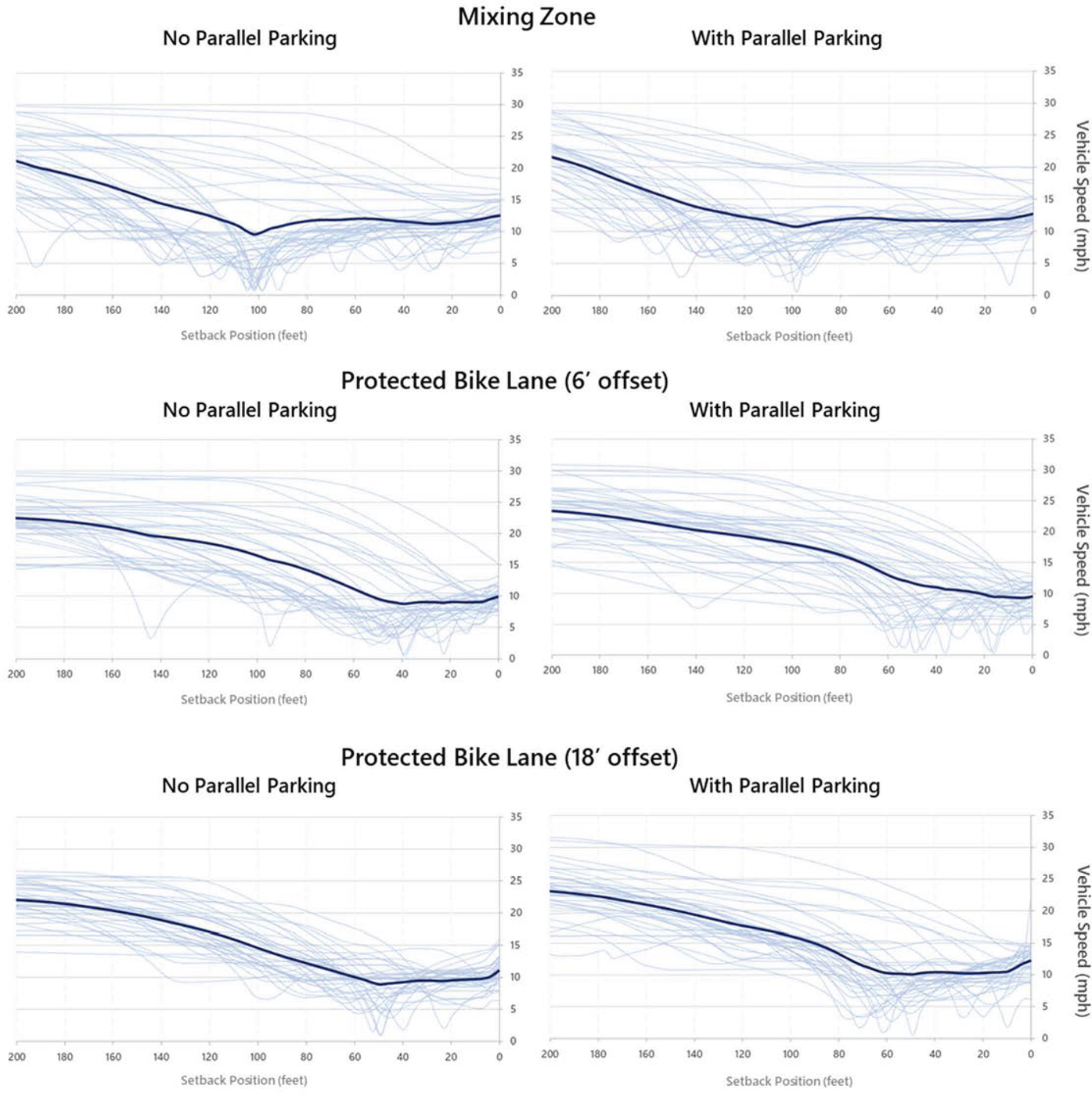
Interestingly, at both protected intersections, average speeds in the transition and turn zones were observed to be higher when parallel parking was present (Figure 52). Regarding the 6-foot offset scenarios, the average transition zone speeds between parallel parking conditions were no PP = 14.6 and with PP = 16.8 mph. Similarly, the average turn zone speeds between parallel parking conditions were no PP = 8.7
and with PP = 10.3 mph. Regarding the 6-foot offset scenarios, the average transition zone speeds between parallel parking conditions were no PP = 13.1 and with PP = 14.3 mph. Similarly, the average turn zone speeds between parallel parking conditions were no PP = 9.3 and with PP = 10.1 mph. Additionally, this was accompanied by notable increases in spread of speeds between parallel parking levels (6-foot Offset: SDno PP = 3.0 vs. SDwith PP = 5.0 mph; 18-foot Offset: SDno PP = 1.3 vs. SDwith PP = 2.5 mph).
A potential rationale for this behavior is the increased workload associated with these geometric conditions, partially due to the parallel parking obstructing the cyclist’s visibility. Maybe less understood is the impact of the buffer’s vertical height and bike lane offset on drivers’ perception of the cyclist’s speed and proximity relative to their location. It is possible that drivers were deterred by the demands of this task and alternatively increased their speeds to enter the intersection far enough downstream from the conflicting cyclist to avoid potential conflict.
Further supporting this variance in driver speeds upon the inclusion of parallel parking at protected intersections are the post-experiment survey responses – there was more variability in the intensity of people’s attitudes towards protected intersections. Remarks typically centered around the physical separation and buffer. Some participants indicated the physical curb buffer negatively impacted their performance, stating it was “harder to check for the cyclists.” A different participant stated that it was difficult to decipher “whether or not a bike would be riding along that path” and in return, “caused me to slow down immensely when turning at intersection in order to confirm that I was not going to hit a cyclist.” One intriguing remark about the protected intersections was,
“The distance from the road makes it feel like the cyclist is riding on a sidewalk, which gives me, the driver, the right of way. So the separated [protected] bike lane lowers my level of confidence to drive safely and avoid collision when a cyclist is adjacent to me.”
These perceptions of the physical buffer and their stated implications on driver safety and speed warrant further investigation into how the spatial construct of the barrier impacts drivers’ perceptions of cyclist’s trajectories and comprehending who has ROW. The inclusion of signing to communicate ROW is also appropriate for future study.
When assessing the combined speed profile and visual attention plots, the difference in driver behavior is illustrated between each intersection type. Worthy of discussion is the comparison of driver speeds and visual attention at the intersections with the conventional and protected intersections. While these two intersections provide drivers with unobstructed visibility of the cyclist, behaviors in terms of speed and visual attention vary not only in magnitude, but in position. With reference to the protected intersections (18’ offset, no parallel parking), more uniformity is observed among driver’s speeds as they approach and traverse the intersection. Notably, drivers were observed to begin decelerating at a further setback from the intersection, and consequently, their rates of deceleration were steadier. Further, between the four intersections plotted, drivers had the lowest speeds overall at a position 200’ back from the turn. In opposition, more erratic deceleration profiles were observed at the intersection with conventional bike lanes. Moreover, there was greater variance between drivers’ speed profiles at the protected intersections, in terms of average speeds per zone. This difference in driver behavior across two intersections with similar geometry, ROW, and cyclist visibility may be derived in the corresponding visual attention on the cyclist.
For the protected intersection scenarios, the greatest percentage of visual attention on the cyclist was allocated in the approach zone, which is the same zone during which many of the drivers began their deceleration into the intersection (some of which started farther upstream, before the start of the approach zone). In opposition, at the intersection with the conventional bike lane, the greatest visual attention on the cyclist occurred closest to the intersection, and secondly, there was less consistency between drivers’ speed profiles, nonetheless, drivers approached the intersections and entered the right-turn maneuver at higher speeds. This finding may suggest that the visual displacement (in the driver’s eye) of the cyclist,
corresponding to shifting the bike lane, may in return yield increased driver awareness of the cyclist. Further, it would be worth investigating the extent to which stimulating driver awareness of a cyclist at a specified distance upstream of the turn (>100’) may promote drivers to make their decision, on whether to yield or not, further upstream of the turn. If this were to be the case, where drivers make their decision farther upstream, the observed consistency in speed profiles and overall deceleration should be further investigated as it serves as a safety benefit. This concept of providing information far upstream of the intersection that is directly relevant to the behavior that needs to occur upon entering the intersection, is already illustrated in the traffic control demand domain by flashing advance warning lights with signage stating, “prepare to stop when flashing.” Above all, the upstream onset of drivers’ visual attention and decreased speeds warrant further exploration in determining if and how the lateral shift of the bike lane served the same purpose of flashing advance warning lights. If they do, how can the geometric design aspects of this human-roadway interaction be manipulated in other intersections to elicit those same driver behaviors and attitudes?


