Protecting Transportation Employees and the Traveling Public from Airborne Diseases (2024)
Chapter: 6 "Closed Box Model" can be Used to Optimize Space to Reduce Virus Transmission
Chapter 6
“Closed Box Model” can be Used to Optimize Space to Reduce Virus Transmission
Methods
This study uses the COVID-19 Aerosol Transmission Estimator tool developed by Jimenez and Peng (2020) during the COVID-19 global pandemic to understand the influences of different factors in the spread viruses on in public spaces. The model was adapted for various public transportation applications. The model is utilized and studied to understand the relative impacts of various factors to the spread of viral contagions in a city bus, light rail unit, and an airplane.
Multivariable regression is used to produce a summary of the influence of each input variable for three types of public transportation vehicles. Reducing the model down to one equation is a useful tool to identify a path forward toward reducing the aerosol transmission risk by quickly identifying which factors to work on. This study also looks at a detailed example of changing transit bus airflow and filtration is analyzed to illustrate an approach and metrics that can be employed to making investment decisions to improve public health. The transmission risks are compared amongst different modes of transport. The transmission risks are also compared to vehicle accident rates to understand how viral transmission risks line up against total travel risk. Finally, recommendations are made regarding the best ways to invest to improve transit vehicle safety overall.
COVID-19 Aerosol Transmission Estimator
Jimenez and Peng (2020) developed this spreadsheet-based risk calculator as an aid to understand what factors influence COVID-19 and aerosol transmission. The COVID-19 Aerosol Transmission Estimator estimates the probability of COVID-19 virus transmission in-between vehicle occupants during a single trip. It uses numerous estimations and multiplies them by several more estimations. The absolute risk level calculated may not be accurate, but the relative improvements when comparing different scenarios are directionally correct. The different input variables are independent. If the model shows that filter A has half the risk as filter B, that one-half ratio will hold even if the number of people on the bus triples. See Table 31 for an example.
Table 31: Independent nature of input variables as it applies to risk of infection.
| 10 Passengers | 30 Passengers | |
| Filter A | Risk = 1 | Risk = 3 |
| Filter B | Risk = 2 | Risk = 6 |
Model Assumptions
These assumptions are inherent to the COVID-19 Aerosol Transmission Estimator and the equations it uses:
- The model estimates the spread of the COVID-19 Omicron B variant by aerosol transmission only.
- It does not estimate transmission by direct physical contact.
- It does not estimate transmission by directly coughing or sneezing on other people.
- It does not estimate transmission by virus deposited on surfaces.
- It calculates transmission risk during a single event. Ex., one bus ride.
Three assumptions were added for transit vehicles:
- Each passenger is on the vehicle more than 5 min.
- The vehicle has HVAC system with the evaporator (recirculation) fan running.
- The vehicle occupants are sitting with minimal talking.
Model Equations
Five primary equations are used in the model. Equation 24 approximates the rate of COVID quanta production and Equation 25 provides a correction for wearing masks. Equation 26 is a mass balance of the airborne quanta based on an atmospheric box model where the air is well mixed throughout the entire space. This is used to calculate the average quanta per cubic meter of air. Equation 27 calculates the quanta dose per person. Equation 28 approximates the risk of contracting COVID-19 for a given quanta inhaled. It is based on the standard Wells-Riley model of aerosol disease transmission.
Notation: A quanta is the amount of virus that, when inhaled, will cause a person to become infected with the virus 63% of the time. Quanta is used as an intermediate step in Equations 24-28.
Equation 24: Quanta Emission Rate
ERq = Cv · Ci · IR · Vd
Where:
ERq = Quanta Emission Rate (Quanta * h-1)
Cv = The viral load in the sputum (RNA copies *ml-1)
Ci = The ratio between one infectious quantum over the infectious dose expressed in viral RNA copies (Quanta RNA copies-1)
IR= Inhalation Rate (m3 · hr-1)
Vd = droplet volume concentration expelled by the infectious person (ml *m-3) (Buonanno et al.)
Equation 25: Mask Correction
NER = ERq * (1-FWF * EME) * NIP
Where:
NER = Net emission rate (Quanta * h-1)
FWF = Fraction wearing facemasks
EME = Exhalation mask efficiency (fraction)
NIP = Number of infected people
(Jimenez & Peng)
Equation 26: Mass Balance of the Quanta Concentration in the Air
Where:
AQC = Average quanta concentration (Quanta * m-3)
TLR = Total Loss Rate (Hr-1)
V= The volume of the indoor environment considered(m3)
t = time (h)
(Jimenez & Peng)
The Total Loss Rate is a combination of several factors that reduce the number of viral quanta in the cabin air. The units are Hr-1, total airflow per hour divided by vehicle volume, or ACH. Facemasks reduce quanta and risk of infection in Equations 25 and 27.
| Total Loss Rate Reduction Factor | Example values for a transit bus with a MERV13 filter |
|---|---|
| Interior air that exits the vehicle | 35.6 /hour |
| Interior air that passes through a filter or germicidal UV *device efficiency | 26.9 /hour |
| Viral aerosol droplets falling slowly to the floor | 0.30 /hour |
| Virus dying over time | 0.62 /hour |
| Total Loss Rate = Sum | 63.4 /hour |
The (1 – e –TLR * t) term in Equation 26 equals approximately 1 in many transit situations. These are the required conditions:
- Each passenger is on the vehicle for at least 5 minutes.
- The transit vehicle is equipped with an HVAC unit and the evaporator fan is running.
Or
A significant fraction of the windows is open, and the vehicle is moving at speed. This scenario is not considered in this report.
Equation 27: Quanta dose per person
QIPP = AQC * BR * t * (1-IME * FWF)
Where:
QIPP = Quanta inhaled per person (Quanta)
AQC = Average quanta concentration (Quanta * m-3)
BR = Breathing rate (m3 min-1)
t = time (h)
IME = Inhalation mask efficiency (fraction)
FWF = Fraction wearing facemasks
(Jimenez & Peng)
Equation 28: Probability of infection from a given viral dose
“Wells-Riley model”
Pt = 1 - e-Dq
Where:
Pt = The probability of Infection. (%)
DQ = The viral dose in quanta. (fraction)
(Buonanno et al.) (Riley et al.)
Model Input Values
The Aerosol Transmission Estimator as received had examples of a subway car, classroom, supermarket, choir practice room, and stadium. It was designed to be adaptable, and new scenarios were created for Bus
A, a Siemens S70 light rail unit, and a Boeing 737-800 airliner by modifying various vehicle size and air handling parameters. The parameters modified for each new scenario are shown in Table 33.
Table 33 shows the range of the input variables across all three forms of public transportation. This is to facilitate comparing relative change of inputs with different units. Each variable was compared to the others by making a change of 10% of the typical value.
| Input Parameters | ||||||||
| # | Bus | Light Rail | Airplane | Source | ||||
| Model | Bus A | Siemens S70 | Boeing 737-800 | |||||
| HVAC | TK T-14 | TK LRV 12T | - | |||||
| Variable | Units | Typical | Typical | Typical | Min | Max | ||
| 1 | Outside air flow | CFM | 1200 | 900 | 1900 | 0 | 1.14 | (5,13,6) |
| 2 | Recirculation air flow | CFM | 1200 | 2600 | 1900 | 0 | 1.14 | (3,13,6) |
| 3 | HVAC Filter efficiency | 1/1 | 0.25 | 0.65 | 1 | 0 | 1 | (x,13,6) |
| 4 | Volume of room | m^3 | 57 | 149 | 142 | 5 | 150 | (5,13,16) |
| 5 | Duration of event | Hour | 0.33 | 0.33 | 1.67 | 0.08 | 1.67 | |
| 6 | Event Repetitions | Count | 1 | 1 | ||||
| 7 | Decay rate of virus | h^-1 | 0.62 | 0.62 | 0.62 | (8) | ||
| 8 | Deposition rate to surfaces | h^-1 | 0.3 | 0.3 | 0.3 | (8) | ||
| 9 | Number of people | Count | 35 | 89 | 178 | 5 | 200 | |
| 10 | Fraction of population immune | 1/1 | 0.35 | 0.35 | 0.35 | 0 | 1 | |
| 11 | Probability of being infective | 1/1 | 0.001 | 0.001 | 0.001 | 0 | 0.1 | |
| 12 | Hospitalization rate | 1/1 | 0.1 | 0.1 | 0.1 | |||
| 13 | Death Rate (IFR) | 1/1 | 0.01 | 0.01 | 0.01 | .00002 | 0.15 | |
| 14 | Breathing rate | m^3/h | 0.8 | 0.8 | 0.8 | |||
| 15 | Relative breathing rate factor | 1/1 | 2.78 | 2.78 | 2.78 | (8) | ||
| 16 | Basic quanta exhalation rate | Q/h | 18.6 | 18.6 | 18.6 | (8) | ||
| 17 | Q enhancement due to variants | 1/1 | 3.3 | 3.3 | 3.3 | (8) | ||
| 18 | Q enhancement due to talking | 1/1 | 1 | 1 | 1 | (8) | ||
| 19 | Mask usage | 1/1 | 0.1 | 0.1 | 0.1 | 0 | 1 | |
| 20 | Exhalation mask efficiency | 1/1 | 0.5 | 0.5 | 0.5 | 0 | 1 | |
| 21 | Inhalation mask efficiency | 1/1 | 0.3 | 0.3 | 0.3 | 0 | 1 | |
Since the model came in the form of a pre-programmed spreadsheet, the inputs were mapped to the main output: the probability of infection. Figure 126 shows a map of the interconnections of the spreadsheet formulas.

The relationships are linear in nature, except for the ones that are labeled (E^x). The exponential components Total First Order Loss Rate and Duration of Event are both well approximated by a linear function in transport vehicles with the following assumptions:
- There is a relatively high HVAC airflow rate for vehicle volume. (>15 ACH)
- Passengers ride for at least 5 minutes.
The exponential component relating Quanta Inhaled per Person to Probability of Infection can be accounted for with a logarithmic transformation before a linear model is calculated.
These assumptions are reasonable for the three applications examined in this study: A transit bus, a light rail car and an airliner. This allows the model to be reduced to a series of linear relationships. This permits the use of a multivariable regression technique to compare the relative impacts of the input variables. These techniques are described elsewhere in the report.
Methods: Multivariable Regression Procedure
A linear least squares regression approach was utilized to reduce the complex relationships to a single formula for comparison purposes. The final formula will take on the generalized form of
Equation 29
y = a0 + a1x + a2z…
Where:
y = The dependent variable
x, z = Independent variables
a0, a1, ax = multiple regression parameters
(Lipson)
The tools and equations to calculate the multivariable regression parameters are designed to work on data sets. In this case, there is no data per se, so a hypothetical data set was created. 120 random variables were created bounded by the ranges shown in Table 33. The net distribution has the mean at the center of the range and a uniform distribution throughout. The sample variation information is ignored, as there is no real data. The seven parameters most applicable for public transit operators were chosen for the regression and are shown in Table 34.
Table 34: Input variable chosen for transit multivariable regression.
| Transit Parameter |
| Fresh air flow rate |
| Recirculated air flow rate |
| HVAC Filter Efficiency |
| Mask Usage Ratio |
| Vehicle Interior Volume |
| Trip Time |
| Number of people in vehicle |
The equations to solve for the 7 regression parameters are large and lend themselves to being solved using statistical computer tools. The equations for a 2-parameter case are shown here for simplicity purposes. Larger parameter equations are calculated in a similar fashion. First, the distance from the mean is calculated for each measurement:
(Equation 30)
(Equation 31)
(Equation 32)
Where:
The sample average of each input
xi, yi and zi = The individual data points
X, Y, Z = The distance from the mean to each data point
(Lipson)
Then, the parameters are calculated using these equations:
(Equation 33)
(Equation 34)
(Equation 35)
(Lipson)
To solve the regression parameters, the online tool Multiple linear Regression Calculator from Statistics Kingdom was used (Multiple Linear Regression Calculator, n.d.-b). The regression was also done by taking the natural log of each individual parameter and the output to determine if there is an improvement of the fit when it is linearized. The goodness of fit was judged by the r2 (multiple correlation coefficient) variable from the following equations (again for the 2-parameter case):
(Equation 36)
= The multiple correlation coefficient of y and x on z
Sy·xz = The standard error of the estimate of y on x and z
Sy = sample standard deviation of y
(Lipson)
The standard error of the estimate is computed from:
(Equation 37)
Where:
n = number of data points
n - 3 = degrees of freedom, determined by the number of parameters estimated (the n’s)
(Lipson)
Bus Blower/Filter Upgrade Cost Calculations
The in-depth example will determine which possible investments a transit authority should select for the largest decrease in viral transmission per dollar of yearly cost. The aerosol model outlined above determines the relative reduction in transmission rate. These calculations, for the yearly cost of making the respective upgrades to the bus, were outlined earlier. Table 35 shows how the yearly fuel costs were calculated for the different options (shown in right column). The example shown is for OEM forward curved blowers in the base configuration.
| Parameter | Multiply | Divide | Options |
|---|---|---|---|
| Blower Shaft Power (W) | 410 | 410 (FC), 335(BC) | |
| Flow Scaling^3 = Power Scaling | 1 | (0.9, 1, 1.1, 1.2) ^3 | |
| Blowers per Bus | 2 | ~ 3.222 | |
| Blower Motor Efficiency | 0.8 | ||
| Alternator efficiency | 0.6 | ||
| Engine efficiency | 0.4 |
| BTU/hr. per W | 3.412 | ||
| Gallons of diesel per BTU | 128,488 | ||
| Dollars per gallon diesel | $4.00 | ||
| Hours per year | 2912 | ||
| Yearly fuel cost | $1,322 |
Table 36 illustrates how the annual cost to change out the blowers was derived. It estimates the annualized cost to change out the constant speed forward curved blowers to attain an airflow change to be $450 a year for a bus with 6 years of life remaining.
Table 36: Cost of upgrading bus Forward Curved HVAC blowers.
| Parameter | |
|---|---|
| Number of Blowers | 6 |
| Cost per Blower (½ the CFM) | $200 |
| Cost Adjustment for Correct CFM | 2 |
| Total Material Cost | $2400 |
| Installation Hours | 3 |
| Labor per Hour | $100 |
| Total Labor | $300 |
| Total Blower Cost | $2700 |
| Average Blower Use after Upgrade (Yrs) | 6 |
| Annual Cost of Upgrade | $450 |
Table 37 shows the assumptions that went into computing the annual filter cost of the two different filter types used in the detailed study:
Table 37: Yearly cost of different filtration levels – MERV 8 and MERV 13.
| MERV 8 | MERV 13 | |
| COVID filtration efficiency | 0.3 | 0.9 |
| Yearly filter changes | 4 | 8 |
| Bulk cost per filter | $12 | $15 |
| Filters per vehicle | 2 | 2 |
| Annual filter cost | $96 | $240 |
Results
Aerosol Transmission Estimator Runs
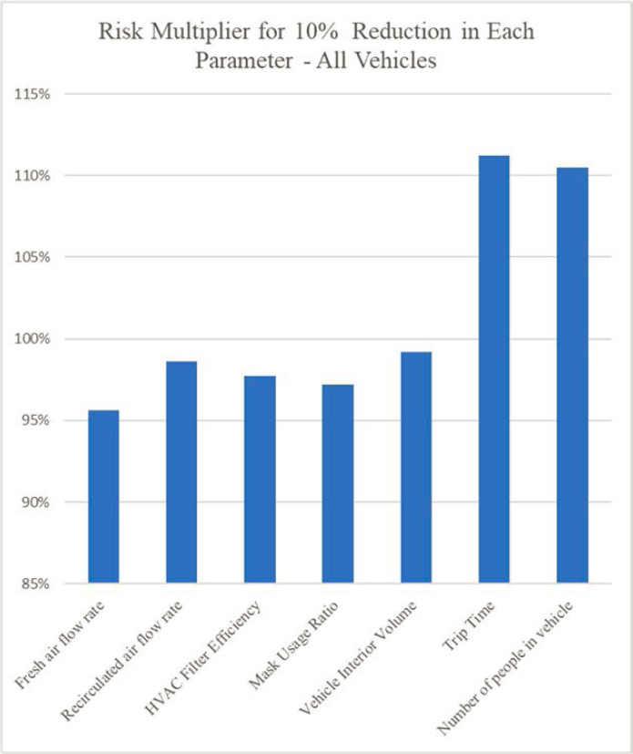
The input variables have different units. They were normalized so their influence on the probability of infection can be understood. This was done by starting with a vehicle typical value and then increasing that value by 10%. This is the partial derivative with respect to each individual input variable at each baseline value. Table 38 and Table 39 and Table 40 show the relative risk multiplier and percent risk change for a 10% increase in each input for the bus, light rail and airplane vehicles respectively.
Table 38: Relative influence of each factor at nominal Bus A values.
| Bus Inputs |
Baseline Value | Units | Relative Risk Multiplier for +10% of Input | % Risk Change for +10% of Input (Negative is Better) |
|---|---|---|---|---|
| Fresh Airflow | 1200 | ft3/min | 0.932 | -6.8% |
| Recirculated Airflow | 1200 | ft3/min | 0.982 | -1.8% |
| HVAC Filter Efficiency | 0.25 | -/- | 0.982 | -1.8% |
| Mask Usage Ratio | 0.1 | -/- | 0.992 | -0.8% |
| Vehicle Interior Volume | 57 | m^3 | 0.991 | -0.9% |
| Trip Time | 20 | minutes | 1.107 | +10.7% |
| Number of People | 35 | number | 1.103 | +10.3% |
Table 39: Relative influence of each factor at nominal Siemens S70 Light Rail Unit values.
| Light Rail Inputs |
Baseline Value | Units | Relative Risk Multiplier for +10% of Input | % Risk Change for +10% of Input (Negative is Better) |
|---|---|---|---|---|
| Fresh Airflow | 900 | ft3/min | 0.975 | -2.5% |
| Recirculated Airflow | 2600 | ft3/min | 0.941 | -5.9% |
| HVAC Filter Efficiency | 0.85 | -/- | 0.941 | -5.9% |
| Mask Usage Ratio | 0.1 | -/- | 0.992 | -0.8% |
| Vehicle Interior Volume | 149 | m^3 | 0.989 | -1.1% |
| Trip Time | 20 | minutes | 1.109 | 10.9% |
| Number of People | 89 | number | 1.101 | 10.1% |
Table 40: Relative influence of each factor at nominal Boeing 737-800 Airplane values.
| Airplane Inputs |
Baseline Value | Units | Relative Risk Multiplier for +10% of Input | % Risk Change for +10% of Input (Negative is Better) |
|---|---|---|---|---|
| Fresh Airflow | 1900 | ft3/min | 0.954 | -4.6% |
| Recirculated Airflow | 1900 | ft3/min | 0.954 | -4.6% |
| HVAC Filter Efficiency | 1 | -/- | - | - |
| Mask Usage Ratio | 0.1 | -/- | 0.992 | -0.8% |
| Vehicle Interior Volume | 142 | m^3 | 0.991 | -0.9% |
| Trip Time | 100 | minutes | 1.101 | +10.1% |
| Number of People | 178 | number | 1.100 | +10.0% |
Table 41 shows a comparison of the relative risk multiplier for each type of vehicle.
Table 41: Relative influence of each factor at nominal values.
| Inputs | Units | Relative Risk Multiplier for +10% of Input | ||
|---|---|---|---|---|
| Bus | Light Rail | Airplane | ||
| Fresh Airflow | ft^3/min | 0.932 | 0.975 | 0.954 |
| Recirculated Airflow | ft^3/min | 0.982 | 0.941 | 0.954 |
| HVAC Filter Efficiency | -/- | 0.982 | 0.941 | - |
| Mask Usage Ratio | -/- | 0.992 | 0.992 | 0.992 |
| Vehicle Interior Volume | m^3 | 0.991 | 0.989 | 0.991 |
| Trip Time | Minutes | 1.107 | 1.109 | 1.101 |
| Number of People | Number | 1.103 | 1.101 | 1.100 |
Regression Approximation of Model
The output formula from the multivariable regression procedure described previously is shown in Eqn 38. The details of the input variables are laid out in Table 42 below.
Equation 38:
Y = 0.0002750 - 0.000000242 * (X1) - 0.000000090 * (X2) - 0.0002828*(X3) - 0.0003129 * (X4) - 0.000000958 * (X5) + 0.000009865 * (X6) + 0.000009830 * (X7)
The multiple correlation coefficient r2 for Equation 38 was only 0.65, which implies the model is not well correlated to a linear model. This is not surprising because of the logarithmic relationship of the number of virus particles inhaled and the risk of infection. A procedure was then employed that took the natural log (ln) of each parameter to yield the regression fit shown in Equation 39. This improved r2 to 0.95. This suggests a good correlation.
Equation 39:
Ln(Y) = -12.46 - 0.4365 · Ln(X1) - 0.1401 · Ln(X2) - 0.2256 · Ln(X3) - 0.2800 · Ln(X4) - 0.0781 · Ln(X5) + 1.121 · Ln(X6) + 1.0461 · Ln(X7)
Equation 39 was then manipulated algebraically to put the final regression fit into a more usable format shown in Equation 40.
Equation 40
Y = 0.000004051 · X1^-0.4400 · X2^-0.1401 · X3^-0.2040 · X4^-0.2799 · X5^-0.07777 · X6^1.118 · X7^1.046
Table 42 provides the details for each input parameter and their respective units. The basic estimation parameter column is compiled from Equation 38 and the improved estimation column is from Equation 40. The final column shows the percent reduction in risk for a 10% increase in the given input parameter (negative is good). This provides a relative sensitivity value for each parameter. Note that these values
compare well to the final column in Table 42, which is another indication of the strong correlation of Equation 39 to the original model.
Table 42: Summary of the correlation parameters and their influence on the risk of infection.
| Transit Parameter | Name | Units | Basic Estimation Parameters | Improved Estimation Parameters | % Risk Change from Regression for +10% Input |
|---|---|---|---|---|---|
| Fresh Airflow | X1 | CFM | -0.000 000 242 | -0.440 0 | -4.4% |
| Recirculated Airflow | X2 | CFM | -0.000 000 090 | -0.140 1 | -1.4% |
| HVAC Filter Efficiency | X3 | Fraction | -0.000 282 8 | -0.204 0 | -2.3% |
| Mask Usage Ratio | X4 | Fraction | -0.000 312 9 | -0.279 9 | -2.8% |
| Vehicle Interior Volume | X5 | m3 | -0.000 000 958 | -0.077 77 | -0.8% |
| Trip Time | X6 | Minutes | 0.000 009 865 | 1.118 | +11.2% |
| Number of People | X7 | Integer | 0.000 009 830 | 1.046 | +10.5% |
| Formula Constant | X0 | Fraction | 0.000 275 0 | 0.000 004 051 | NA |
| Risk of Infection | Y | Fraction | NA | NA | NA |
Figure 127 shows the relative influence of each of the input parameters. Each parameter is increased 10% and the change in the risk of infection is shown. The graph shows that the most impact can be made by reducing the trip time or the number of people on the vehicle.
Although this regression was originally calculated for the case of a transit bus, it turns out that because of the way that because of the way the inputs were normalized, the same regression model (Equation 38) works for all three types of mass transit vehicles – transit bus, light rail and airplane. So, Figure 127 is applicable for all three modes of transport.
Engineering Improvements
From a practical engineering standpoint, the most likely way to make an impact on viral transmission is to modify the bus HVAC system. This section will focus on transit bus application and examine several scenarios that modify the bus HVAC to reduce transmissions rates in the most cost-effective manner. Three scenarios are considered for Bus HVAC systems with:
- Forward curved evaporator blowers without speed control using improved filtration.
- Replace the forward curved blowers with new ones that offer more effective airflow and improve filtration.
- Backward curved evaporator blowers with speed control and increase the blower speeds / airflow.
- Backward curved evaporator blowers with speed control – changing blowers speeds and improving filtration.
The COVID-19 Aerosol Transmission Estimator tool was used to calculate the transmission risks based on varying the recirculation airflow and filter efficiency based on the different scenarios examined. A basic model was developed to determine the influence of the blower speeds and HVAC system efficiency on bus fuel economy. Costs were estimated from available online resources and are outlined elsewhere.
Transit Bus Scenario 1 – Forward Curved Blowers without Speed Control: Improve Filtration
This first scenario assumes that a given rooftop transit bus has the more compact forward curved blowers installed that do not have variable speed. The issue that comes up with this approach is that the better filter will increase static pressure drop in the HVAC system. This will reduce the recirculation airflow in the bus and reduce the potential amount of air that circulates through the filter, reducing the overall filter system effectiveness. The net improvement in filtration and viral transmission will therefore be net of these offsetting parameters.
This scenario changes from a MERV 8 filter to a higher efficiency MERV 13 filter in the bus HVAC system. The MERV rating refers to a filter’s ability to capture larger particles between 0.3 and 10 microns (µm). The relative ability of the filtration level of these two ratings is shown in Table 43. The MERV 13 filters are much more effective at filtering out virus particles, which are often in the .5 - 10 Micron range.
| MERV Rating | Average Particle Size Efficiency in Microns |
|---|---|
| 8 | 1.0 - 3.0 greater than or equal to 20% 3.0-10.0 greater than or equal to 70% |
| 13 | 0.30-1.0 greater than or equal to 35% 1.0 - 3.0 greater than or equal to 80% 3.0-10.0 greater than or equal to 90% |
This scenario uses the more effective MERV 13 in place of MERV 8 filters that increase the flow resistance and lower the airflow by 10%, as described in the relationship between filter pressure drop, IAQ, and energy consumption in rooftop HVAC units. (Zaatari et al). The bus fuel consumption will increase somewhat because the reduced airflow will lower the HVAC system’s efficiency. (Zaatari et al). The cost of the filters was estimated from the information presented elsewhere. Refer to Table 44 to understand the impact of this change scenario.
| Yearly Cost Basis | Baseline Forward Curved Blower | Upgrade To MERV 13 Filter |
|---|---|---|
| Filter MERV Rating | 8 | 13 |
| Blower Type | Forward Curved | Forward Curved |
| Air Flow Change | 0 | -10 % |
| Fuel Cost $ | 1322 | 1584 |
| Filter Cost $ | 96 | 240 |
| Final Total Cost $ | 1418 | 1824 |
| Relative Cost | 1 | 1.29 |
| Risk Ratio | 1 | 0.73 |
| $/year for 10% risk reduction | - | $151 |
The table shows that the yearly cost of running the transit bus will go up $176 due to increased filter cost, more filter changes and lower HVAC efficiency impacting bus fuel economy. The Risk Ratio parameter is the relative risk of infection from the upgrade based on the Aerosol estimator tool. The risk is reduced by 27%. The final row shows the yearly cost of a 10% risk reduction with this approach. This is a way to judge the cost effectiveness of the different approaches.
Transit Bus Scenario 2 – Forward Curved Blowers without Speed Control: Increase Airflow by Replacing the Blowers and Improve Filtration.
This second scenario changes out the forward inclined blowers to gain back the airflow that was lost because of the filter upgrade. Increasing the airflow by 10% was also examined, as shown in Table 45. It includes the cost of installing six new blowers per bus depreciated linearly over 6 years.
| Yearly Cost Basis | Baseline Forward Curved Blower | Upgrade filter & No Airflow Change (New Blowers) | Upgrade filter & + 10% Airflow (New Blowers) |
|---|---|---|---|
| Filter MERV Rating | 8 | 13 | 13 |
| Blower Type | Forward Curved | Forward Curved | Forward Curved |
| Air Flow Change | 0 | 0 | +10 % |
| Fuel Cost $ | 1322 | 1885 | 2496 |
| Filter Cost + Blower Cost $ | 96 | 690 | 690 |
| Final Total Cost $ | 1418 | 2575 | 3186 |
| Relative Cost | 1 | 1.80 | 2.25 |
| Risk Ratio | 1 | 0.70 | 0.67 |
| $/year for 10% risk reduction | - | $377 | $531 |
Transit Bus Scenario 3 – Backward Curved Blowers with Speed Control: Increase Airflow by Speed up the Blowers.
This scenario uses another common evaporator blower configuration on transit buses: backward curved blowers with speed control. The approach here will be to increase the fan speed (and airflow) by 10% and 20% to understand to understand the reduction that is possible without adding better air filters. Increasing the air circulating through the existing filter will lower the number of viral particles in the bus. Speeding up the fans should improve the HVAC cooling potential slightly. However, since the fan laws dictate that the power consumed by a blower goes up with the cube of the speed and the volume flow is only linear, the net affect will be more power consumed from the bus engine. See the equations below.
Equation 41: First Fan Law: Volume Flow
Equation 42: Third Fan Law: Power
Where:
Q1 and Q2: are the volumetric flow from the fan before and after the speed change (CFM)
V1 and V2:are the fan velocity before and after the change (RPM)
P1 and P2:are the fan power consumption before and after the speed change (Watts)
(Admin)
Table 46 shows the results of the calculations. The total cost increase is quite dramatic. The cost for a 10% risk reduction is also quite poor compared to the other scenarios covered so far.
| Yearly Cost Basis | Baseline Backward Curved Blowers | + 10% Fan Speed | + 20% Fan Speed |
|---|---|---|---|
| Filter MERV Rating | 8 | 8 | 8 |
| Blower Type | Backward Curved | Backward Curved | Backward Curved |
| Air Flow Change | 0 | +10 % | +20 % |
| Fuel Cost $ | 1082 | 1440 | 1871 |
| Filter Cost $ | 96 | 96 | 96 |
| Final Total Cost $ | 1178 | 1536 | 1967 |
| Relative Cost | 1 | 1.30 | 1.67 |
| Risk Ratio | 1 | 0.98 | 0.97 |
| $/year for 10% risk reduction | - | $1,989 | $2,254 |
Transit Bus Scenario 4 – Backward Curved Blowers with Speed Control: Improve Filtration and Vary Airflow
This scenario assumes that a MERV 8 bus filter is switched out to a MERV 13 filter, as was done in scenarios 1 and 2. Refer to Table 47. The middle column shows the calculations for the case where the airflow is not adjusted, and the airflow falls 10% because of the increased static resistance to the fan from the filter. The next column shows what happens when the airflow is increased back up to the baseline level. The last column shows the situation when the airflow is increased 10% beyond the baseline.
| Yearly Cost Basis | Baseline Backward Curved Blowers | Upgrade filter & - 10% Airflow | Upgrade filter & No Airflow Change | Upgrade filter & + 10% Airflow |
|---|---|---|---|---|
| Filter MERV Rating | 8 | 13 | 13 | 13 |
| Blower Type | Backward Curved | Backward Curved | Backward Curved | Backward Curved |
| Air Flow Change | 0 | -10 % | 0 | +10 % |
| Fuel Cost $ | 1082 | 1344 | 1475 | 1914 |
| Filter Cost $ | 96 | 240 | 240 | 240 |
| Final Total Cost $ | 1178 | 1584 | 1715 | 2154 |
| Relative Cost | 1 | 1.34 | 1.46 | 1.83 |
| Risk Ratio | 1 | 0.73 | 0.70 | 0.67 |
| $/year for 10% risk reduction | $151 | $177 | $293 |
The lowest cost for a 10% risk reduction is to upgrade the filter and let the airflow decrease. If that is not desirable from an HVAC performance standpoint, raising the airflow up to the initial level is almost as efficient from an investment standpoint ($151 vs $177 for a 10% risk reduction). Speeding up the blowers more than that is increasingly less cost efficient.
Transit Bus Scenarios – Summary
The main deciding factor for which case of each scenario to recommend is based on the Dollars / Year for a 10% percent risk reduction. The assumption is that a given city transit authority has a fixed budget that it can invest to reduce the risk of virus transmission and it will choose to make the most effective investment with the fixed funds that are available. Table 48 summarizes the lowest Dollars / Year for a 10% improvement for each scenario.
| Blower Type | Scenario Number | Increase in yearly operating cost ($) | Corresponding Risk Ratio |
|---|---|---|---|
| Forward Curved, Constant Speed | 1 | $406 | .73 |
| 2 | $1147 | .70 | |
| Backward Curved, Variable Speed | 3 | $406 | .98 |
| 4 | $537 | .73 |
Discussion: Aerosol Transmission Estimator Runs
Reviewing Table 49 shows the Infection Risk Multipliers for the different parameters are relatively similar in between vehicle types. The relatively ineffective MERV 8 filter on the bus makes fresh air more effective than recirculated air at reducing virus transmission. The airplane starts with a HEPA filter that makes recirculated air just as effective as fresh air. Also, changing mask usage from the base value of 10% to 11% has a risk change roughly in line with the absolute change of 1% of people wearing masks. Changing the interior volume of the vehicle has a surprisingly small effect on the risk of air born virus transmission. Trip time and number of people per vehicle have a large effect with +10% of either resulting in approximately 10% more risk. Increasing route frequency is an effective, but expensive, method to reduce risk.
Table 49: Relative influence of each factor at nominal values.
| Inputs | Units | Relative Risk Multiplier for +10% of Input | ||
|---|---|---|---|---|
| Bus | Light Rail | Airplane | ||
| Fresh Airflow | ft^3/min | 0.932 | 0.975 | 0.954 |
| Recirculated Airflow | ft^3/min | 0.982 | 0.941 | 0.954 |
| HVAC Filter Efficiency | -/- | 0.982 | 0.941 | - |
| Mask Usage Ratio | -/- | 0.992 | 0.992 | 0.992 |
| Vehicle Interior Volume | m^3 | 0.991 | 0.989 | 0.991 |
| Trip Time | minutes | 1.107 | 1.109 | 1.101 |
| Number of People | number | 1.103 | 1.101 | 1.100 |
Discussion: Regression Approximation of Model
As can be seen in Figure 128, the Regression Approximation is a relatively good surrogate for each of the vehicle types.
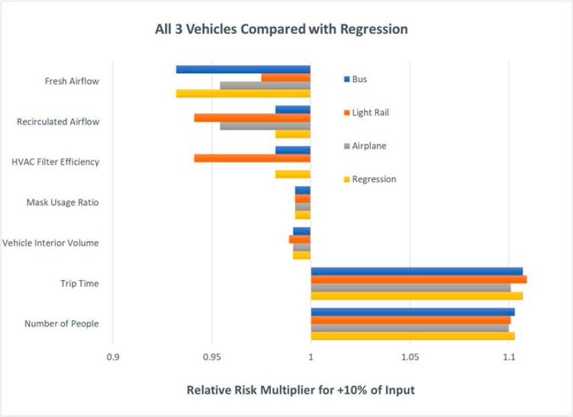
The formula (Equation 40) is more portable than the entire Aerosol Transmission Estimator tool and has the advantage that it is aligned well with public transportation vehicles. It helps decision makers understand the specific situation by providing one formula to inspect.
Engineering Improvements
An examination of which cases yielded the highest return on investment, measured by Dollars / Year for a 10% risk improvement, shows it is most cost-effective to install better filtration and let the airflow
decrease by 10%. (See Table 48) This is the case for both blower types. This will decrease the risk by 27%, which is substantial. If it is deemed unacceptable to reduce the airflow in the bus by 10% for HVAC performance reasons, restoring original airflow with increased speed on variable speed fans is an alternative that costs $131 more per year for a 3% additional reduction in risk of infection (Table 49 and Table 50). In the case of constant speed blowers, the airflow can be brought back up to the original level by replacing blowers, which will cost an additional $769 per year for the same 3% reduction in risk of infection. The reduced infection ratio does not improve substantially.
Table 50: Comparison of select bus filter blower options.
| Blower Type | Airflow Reduction (%) | $ /Year over baseline | Risk Ratio |
|---|---|---|---|
| Forward Curved, Constant Speed | -10 | $406 | 0.73 |
| 0 | $1,147 | 0.70 | |
| Backward Curved, Variable Speed | -10 | $406 | 0.73 |
| 0 | $537 | 0.70 |
Recommendations for Transit Buses
The most cost-effective method for reducing aerosol virus transmission on public transit vehicles is upgrading cabin filters. This is followed by increasing recirculation air flow and then increasing route frequency. Increasing route frequency is not cost-effective when only aerosol viral transmission is considered. The costs in Table 51 reflect the total expense of operating a vehicle including direct expenses, vehicle and non-vehicle maintenance, and general administration. Not all these costs scale exactly 1:1 with vehicle miles, but it is a valid estimation with city and rapid bus fleet miles correlating to total operating cost with an r2 of 0.8. The operating costs increases proposed in this paper are relatively small compared to the overall vehicle operating cost. Higher route frequency may make sense if the route was almost eligible for a frequency increase before viral transmission was considered.
| USA Averages for 2021 | Yearly Operating Cost / Vehicle | $/Year for 10% Risk Reduction | Hours / Vehicle | Miles / Vehicle |
|---|---|---|---|---|
| City Bus, Rapid Bus | $495,000 | $49,500 | 3,130 | 170,770 |
| Light Rail Unit | $1,730,000 | $173,000 | 4,570 | 72,930 |
Filter efficiency reaches a limit of 100%. Increasing airflow only has soft limits that are less well defined. Increasing airflow to the extreme, tripling airflow with upgraded blowers appears more cost-effective than increasing route frequency. This is despite the blower power use scaling with the cube of airflow to 18kW and requiring the purchase of a larger alternator. Tripling the airflow would run into a soft limit where it is unpleasant for passengers. The maximum comfortable airflow should be investigated.
The risk reduction ratios calculated apply for other diseases that spread through aerosol droplets. Distributing optional free facemasks when boarding may also be cost-effective, but this would slow down the boarding process and the associated costs were not investigated in this report. The Federal Highway Administration evaluates safety improvement projects at the rate of $6.20 capital cost per 1 one millionth of a life saved as of 2011. Converting this to a yearly basis with a perpetual annual rate of return of 7%, this corresponds to $0.39 per year per trip. If the current risk of aerosol COVID transmission was 0.02% or 1:5000, the average risk of an infected person dying was 1%, and 40,000 trips per vehicle per year, this would correspond to $3,120 per year for a 10% risk reduction ratio. $3,470 per year covers all the filter and blower upgrade options proposed in this paper.
The risk of death for one trip in a private automobile is about .000 000 75. This is based on National Safety Council (NSC) data from 2021 and assumes traveling by car 1/2 of the days during a 75-year lifespan. Taking the estimated values from the bus baseline case, this would make public transit 2.3 times deadlier per trip, crash risk plus infection risk, than private automobile travel. This risk of death from a public transit vehicle crash is 24 times lower than a private automobile on a per mile basis, based on the same NSC data. This suggests that virus transmission will remain the most dangerous part of traveling on public transit long after the COVID-19 pandemic ends.
Other Important Factors for Public Transit
Newer, more energy efficient buses often have reduced air leaking in and out of the cabin. This will decrease HVAC power requirements but increase the risk of viral transmission.
The box mixing model used does not account for virus transmission by viruses deposited on surfaces, direct physical contact, or directly coughing or sneezing on another person. This model will underestimate the risk when these factors are added in, especially in crowded vehicles.
Age is an important parameter that is not in the model. The risk of death given that you are infected with COVID-19 is heavily age dependent. Thus, it matters if the vehicle is a school bus or a retirement home bus. A senior is at over 1000 times the risk of a 10-year-old. Parents have a 20-40 times higher risk of death than their kids. Age has a much larger effect than any currently known engineering improvements. A retirement home bus could theoretically justify spending 10 times more than a typical transit bus on aerosol virus transmission risk reduction.
Equation 43:
IFR = .000537 ·.0534A
Where:
IFR = Infection Mortality Rate
A = Age in years
(Levin et al)
Final Thoughts
The COVID-19 Aerosol Transmission Estimator is a flexible tool that can be applied to a wide variety of applications, including classrooms, offices, supermarkets, indoor choir practice, restaurants, and vehicles. It is helpful to use multivariable regression techniques to isolate equations for specific applications to understand which variables are most important. This study has shown that there is a clear sequence of upgrades that minimizes the spread of aerosol viruses in public transportation vehicles for several levels of investment. The sequence is first upgrade to a MERV13 or better filter, second increase airflow, and third increase route frequency.


