Protecting Transportation Employees and the Traveling Public from Airborne Diseases (2024)
Chapter: 3 Experimental Studies with Transit Buses
Chapter 3
Experimental Studies with Transit Buses
Methods
Generation and dispersion of COVID-like test aerosol
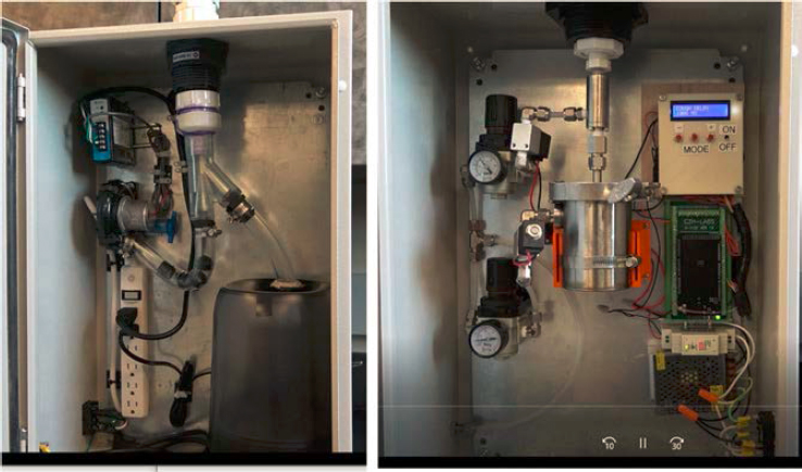
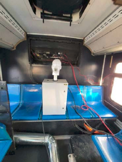
Three aerosol generators were designed, manufactured, and evaluated (Figure 1). The continuous generator produces a continuous stream of NaCl particles. The size of the particles is determined by the NaCl concentration in water. The cough generator produces “puffs” of particles at a frequency and duration set by the user. The third generator is not shown. It produces a high concentration of particles using an ultrasonic technique.
Acquisition and Preparation of the Test Bus
The team acquired two buses for this project. Bus A, in Figure 2 is an in-house bus which was borrowed from CE-CERT’s previous research on a hybrid bus project. Bus A was used to conduct baseline testing. Bus A was modified to conduct Task 2 specifically for the parallel air ventilation system. Bus B, in Figure 3 was borrowed from the LA Metro for this project. This bus was used to conduct a portion of Task 2. It was especially used for a test with passengers on-board. Bus B was used for on-road testing.
Table 1 and Table 2 show specifications of both buses.
Table 1: Bus A Test Vehicle Specifications.
| Vehicle Type | Transit Bus |
|---|---|
| Gross Vehicle Weight Rating (GVWR) | 40,600 lbs |
| Fuel Type | Hybrid – CNG |
| Cabin Volume | 57.25 m3 |
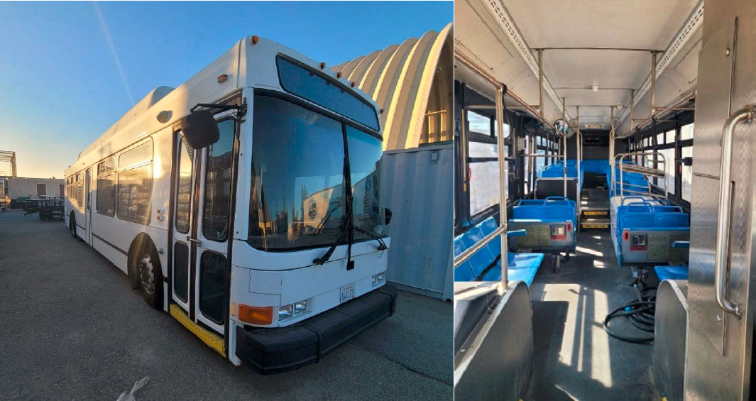
Table 2: Bus B Test Vehicle Specifications.
| Vehicle Type | Transit Bus |
|---|---|
| Gross Vehicle Weight Rating (GVWR) | 30,130 lbs |
| Fuel Type | CNG |
| Cabin Volume | 71.15 m3 |

The bus HVAC system includes filters that impact the movement of airborne particle concentrations inside the cabin and thus virus transmission. The goal is to reduce airborne particle concentrations (i.e., airborne COVID-like aerosol concentrations) via multiple approaches. The experimental approaches used in this study are divided into two groups: Retrofit and redesign as shown by the flowchart in Figure 4. The
retrofit category modifies the bus cabin to examine the effect of plexiglass barriers, effect of air exchange rate, high efficiency cabin filter, and distributed air cleaners. The redesign approach uses a parallel flow system constructed inside Bus A test bus which is detailed later in this report. The parallel system is composed of two blowers that recirculate bus cabin air vertically. The existing ventilation air duct in the back of the bus was disabled and blocked. The blowers supply cabin air to the roof ducts at the left and right sides of the bus so that air can be blown down vertically. There are multiple parallel air outlets with registers placed on the floor of the bus. Each outlet is in a rectangular shape, and it has a MERV 13 filter installed to remove particles. For actual implementation of the parallel system, the design can be much simpler. A duct or ducts can be installed underneath the bus, and it (or they) can be connected to a blower located at the back of the bus. This method is expected to add minimal flow resistance to the bus ventilation system.
Ten TSI AirAssure (8144-2) IAQ monitoring sensors were placed on each seat handle at a height approximately 34 in from the bus cabin floor. The sensors monitor carbon dioxide (CO2) levels, total volatile organic compounds (tVOC), PM, barometric pressure, temperature, and relative humidity. Testing was conducted in laboratory settings to evaluate accuracy and repeatability of sensors which is detailed in Appendix A: Laboratory Tests.
The following subsections will describe the progress completed within each experimental approach. The final subsection contains the test matrix of trials completed thus far for both Bus B and Bus A.

Plexiglas Barriers
Divider barriers were constructed using 1-inch square aluminum tubing connected with 3D printed fittings to form a rectangular frame. The frames varied in height between 2 ft 10 in and 3 ft 4 in depending on the position within the bus they were located as they were limited by the ceiling handlebars. General
lengths were measured at 33.5 inch with a depth of 1 inch. The frames were fitted with a polyester sheet (instead of Plexiglas due to lighter weight, lower cost, and easiness to handle) and they were mounted to the back of each seat, as seen in Figure 5. A total of ten barriers were installed on each seat facing forward to create partitions throughout the cabin of Bus A. The layout of the barrier locations is shown in Figure 6.

Effect of Door Opening
To determine the effect of door opening on air exchange rates and particle concentrations, five different scenarios were tested. The first scenario type includes a baseline test with both the rear and front doors in a closed configuration. The second scenario tests the effect from both doors being in an open configuration to simulate passenger loading and unloading. To determine the effect from each door independently, the next two scenarios test the front door open while the rear door is maintained in a closed configuration and the rear door open while the front door is maintained closed. Lastly, to replicate the effect of air flow while the bus is driving throughout city routes, a Hartzell Series 23 utility air circulating fan was faced towards the bottom of the front door while both doors were closed (Figure 7). As there is a door gap with the floor and air is viscous, the wind may pull cabin air out of the bus cabin increasing air exchange rate.

To compare air changes per hour (ACH) a.k.a. AER (Air Exchange Rate) between each scenario, CO2 canisters were released throughout each bus cabin while ten TSI AirAssure sensors measured CO2 gas decay over time. The rate was calculated by fitting the measured CO2 decay to Equation 1 (Jung et al. 2017). Coefficients A, B, and C were determined by fitting to the measured CO2 levels reported from each sensor. Variable A represents the CO2 concentration at t = 0, B is the background CO2 concentration in ppm, and C is represented as the inverse of the time constant in Equation 2 (based from Jung et al. 2017). C is equal to the AER represented in hr-1. The Matlab2023 Curve Fitter Toolbox application was used to perform a non-linear regression fit to determine each constant. The constants’ constraining bounds are described in Table 3. The constant A was limited to values between 0 to 3000 ppm to represent an initial concentration value for each test. Constant B had a lower bound of 300 ppm based on sensor sensitivity from estimated background concentrations of 420 ppm up to 500 ppm. Constant C was allowed to vary without bounds to obtain the best fit line. The best fit was determined using the selected baseline sensor #4 (refer to Appendix A: Laboratory Tests) and used the Least Absolute Residual method. A fit with the lowest sum of squared estimate of errors and highest adjusted r2 value was selected for the evaluation of the remaining sensors.
Ccabin(t) = (A-B)exp(-Ct)+B (Equation 1)
(Equation 2)
Table 3: Coefficient Constraints of the non-linear CO2 regression analysis using MatLab2023.
| Variable | Lower Bound | Upper Bound |
|---|---|---|
| A | 0 ppm | 3000 ppm to + Inf |
| B | 300 ppm | 420 to 500 ppm |
| C | -Inf | + Inf |
Effect of Cabin Air Filtration Improvements
Each bus HVAC system was equipped with a pre-used MERV 13 filter across the inlet. To evaluate the effectiveness of implementing cabin air filtration improvements a baseline test was conducted to compare results using the existing filter with no modifications. In this phase of testing, the aerosol generator was powered on to increase PM concentration within the cabin and then powered off to allow for the PM concentration to decay through filtration and particle deposition loss to the walls. The aerosol generator was placed in the front, middle, and back seats of the cabin to test varying source locations inside the cabin. Particle count and size distributions were measured using a TSI 3080 electrostatic classifier and 3776 CPC. An eACH (Equivalent ACH) value is calculated by fitting the exponential PM decay over time after the aerosol generator is powered off. The time constant represented by Equation 2 represents the particle removal rate and is used to compare between tests. A new electrostatically charged ThermoKing MERV 13 filter (46 in x 20.6 in) was installed to compare to the in-use pre-used MERV 13 filter and review the efficiency of PM removal.
Effect of On-board Air Cleaners
Prior to replacement of the pre-existing MERV 13 filter equipped in each bus HVAC system, the effect of on-board standalone air cleaners was tested. The modifications included the use of two Honeywell HEPA air purifiers (model HPA300) with a flow output of approximately 320 CFM air flow on the “turbo” setting, in tandem with the bus AC system after the aerosol generator is powered off. This method affects the rate of PM decay which can be compared to the baseline scenario. One of the HEPA air purifiers was placed near sensors #1-4 located at the front section of the bus cabin, while the second HEPA air purifier was placed near sensors #5-8 located at the back of the cabin. The aerosol generator was placed in the front, middle, and back of the cabin to also test varying source locations within the cabin.
Effective of Ventilation Design Changes
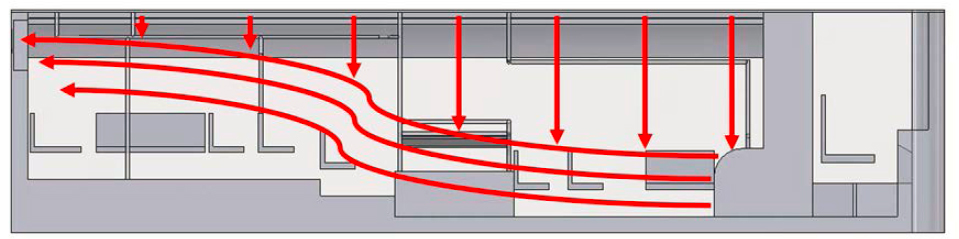
A standard transit bus has a ventilation system which operates by supplying air into the bus cabin through two vents which run along the corners of the ceiling of the bus’s cabin, supplying air throughout most of the bus’s length. As seen in Figure 8, air inside the cabin is first removed through an extraction fan in the rear of the bus, causing the need for air to move across the entire length of the bus prior to being removed. If someone in the front seat coughs, then the virus aerosol can be transmitted to passengers in the back seat easily following this type of ventilation air flow.
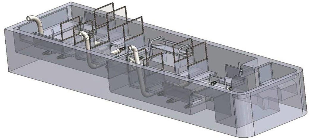
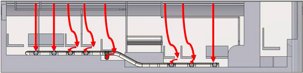
The proposed parallel ventilation system, depicted in Figure 9, combines the standard upper ventilation system with a lower system which replaces the function of the extraction fan located at the rear to remove air from the bus. Figure 10 shows this lower ventilation system which consists of 17 vents that branch into each row of seats removing air throughout the length of the bus. Each branch is capped with a register box.

A dual blower system, consisting of two three-phase 5HP motors and PB15A Cincinnati fans, creates a closed loop system in which air is being cycled from the outlet of each blower to the upper ventilation system while air is being removed through the lower ventilation system which is led into the blower inlets. A variable frequency drive is what controls the motor and fan, enabling flow rate adjustments in the lower
ventilation system. To achieve the desired flow rates in both the upper and lower ventilation systems, the two blowers were set at maximum speed of 3600 rpms. As seen in Figure 11, the outlets of these blowers, shown in red arrows, are connected to two points which supply air to both sides of the upper ventilation system. The inlets of these blowers, shown in blue arrows, are connected to three points in the lower ventilation system for active air removal from inside the bus cabin.
Figure 12 shows images of the dual blower system installed onto Bus A. The current configuration of the dual blower system is only to facilitate the demonstration of the parallel system without major redesign or re-construction of the bus cabin HVAC system. In real application, if a bus manufacturer would like to implement the parallel ventilation system, then they simply need to run one or two rectangular channels (like the already existing ones at the corners of the ceiling) under the floor of the cabin and circulate the air by designing and placing a blower in the back of the bus connecting the two top channels with the bottom channel as shown in Figure 13. Inlets of the cabin air can be made by putting grilles on the cabin floor.


Determine Effect of “Clean Air Shower System”
This task is functionally the same as the task described above (2.2.5). An air shower technique in stationary test used only ventilation slots from roof vents located directly above floor suction vents. Specifically, the roof ventilation contains multiple air slots of 50.51 mm, width of 9.87 mm, and straight length of 44.62 mm (Figure 14) throughout the length of the vent duct. The slots that were not directly above the floor suction vents were sealed.

On-road Testing
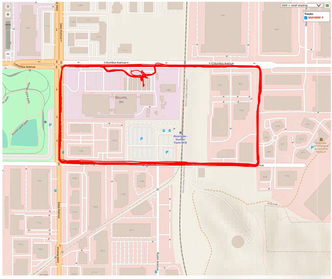
The use of on-road testing provides realistic driving conditions experienced by bus operators and a traveling public. On-road testing incorporates the identical sensor and aerosol generator placement set up used in the stationary testing. A baseline test was performed without the use of the aerosol generator to determine backline conditions. A map of the on-road test pathway is shown in Figure 15 and measures approximately 1.11 miles in perimeter and is composed of 35 mph to 45 mph roads to mimic the driving pattern of a public transit bus. Driving patterns for each test include 2-3 continuous laps around the test pathway, showing repeatable driving patterns throughout the speed profiles (Figure 16). Ambient conditions during two testing days included an average temperature of 81.65 °F and 77.89°F and maximum wind speeds of 14 mph and 17 mph.

Test Matrix
Table 4 shows the test matrix for ACH/AER testing using CO2 canisters. Decay rates of CO2 concentrations were used to determine ACH at different test conditions. All windows and roof latches were maintained in a closed position for all tests in this study. CO2 canisters were released throughout the bus cabin and the concentration was allowed to decay within each test. The opening and closing of the bus doors were used to test different air exchange conditions including opening both doors, opening only one door, and both doors closed. In addition, a Hartzell Series 23 utility air circulating fan was used to simulate driving conditions with air flow outside the cabin.
Table 5 shows the test matrix of the eACH testing using a particle generator during stationary testing with the regular bus HVAC system. The eACH value for particles removed were determined from the decay rates of particle concentrations at multiple locations of the bus cabin for different test conditions. The aerosol generator was placed at three locations: at the front of the bus in the seat facing perpendicular to the center aisle, middle of the bus near sensors 5 & 6, and center of the back row seat against the back wall of the cabin, see Figure 17. The generator was powered to allow the particle mass concentration to reach an approximate plateau before turning off allowing for the concentration to decay. A variety of experimental conditions used include installing plexiglass barriers to create partitions inside the cabin, and the use of standalone HEPA air purifiers.
Table 6 shows the test matrix of eACH testing during stationary testing with the parallel ventilation system. The aerosol generator is also placed at the same three locations throughout the bus, and experimental conditions include the use of barriers, and an air shower method described later.
Table 7 shows the test matrix during stationary testing using a new MERV 13 filter replacement to determine particle removal and filter efficiency.
Table 8 provides a summary of the test matrix used for on-road testing. The stop-and-go experimental condition signifies minimal traffic roads containing stop signs and traffic signals.
The aerosol generator was powered on until the particle mass concentration stabilized to a plateau, replicating stationary testing. The bus AC system was set to high and in a stationary position. CO2 canisters
were then released throughout the cabin before the driver entered the bus. The maximum cabin CO2 reached about 2000 ppm. While this is not a harmful level for a short exposure, the driver was recommended to wear an adsorption type gas mask (JOEAIS 6200 respirator) as a precaution. Upon releasing CO2, the aerosol generator was turned off, the driver waited 3-5 min for mixing and started driving the test pathway. Each test includes 2-3 laps through the pathway which included stop signs, traffic signals, and minimal traffic with speeds of 35 to 45 MPH. The stop-and-go test incorporated six laps around the test pathway with stopping at the end of each lap with the doors open for an interval of 20 to 40 seconds to simulate passenger loading and unloading.
Table 4: Stationary test matrix using CO2 gas with conventional ventilation system
| Test # | Amount of CO2 Gas Released (g) | Air Exchange Type | AC Fan | Driver Fan |
|---|---|---|---|---|
| Bus B | ||||
| 4 | 150 | Doors closed | Hi | - |
| Front door open | Hi | - | ||
| 6 | 150 | Doors closed | Hi | Hi |
| 7 | 150 | Doors closed | Hi | Lo |
| 8 | 171 | Dyno Fan blowing over the closed front door | Hi | - |
| Both doors open | Hi | - | ||
| 13 | Passenger | Doors closed | Hi | - |
| Doors closed | Hi | Hi | ||
| Doors open | Hi | Hi | ||
| Bus A | ||||
| 10 | 150 | Doors closed | Hi | - |
| 11 | 150 | Doors closed | Hi | - |
| Doors open | Hi | - | ||
| 12 | 150 | Dyno Fan blowing over the closed front door | Hi | - |
| Rear Door open | Hi | - | ||
| 13 | 150 | Dyno Fan blowing over the closed front door | Hi | - |
| Front Door open | Hi | - |
| Test # | Aerosol Generator Location | Experimental Condition | AC Fan | Driver Fan |
|---|---|---|---|---|
| Bus B | ||||
| 1 | Front Seat | Baseline | Off | - |
| 2 | Front Seat | Baseline | Hi | - |
| 3 | Middle Seat | Baseline | Hi | - |
| 9 | Front Seat | HEPA Filters | Hi | - |
| 10 | Front Seat | Baseline – Repeat | Hi | - |
| 11 | Middle Seat | HEPA Filters | Hi | - |
| 12 | Middle Seat | Baseline – Repeat | Hi | - |
| Bus A | ||||
| 1 | Front Seat | Barriers | Hi | - |
| 2 | Middle Seat | Barriers | Hi | - |
| 3 | Back Seat | Barriers | Hi | - |
| 4 | Front Seat | Barriers + HEPA | Hi | - |
| 5 | Middle Seat | Barriers + HEPA | Hi | - |
| 6 | Back Seat | Barriers + HEPA | Hi | - |
| 7 | Back Seat | HEPA Filters | Hi | - |
| 8 | Middle Seat | HEPA Filters | Hi | - |
| 9 | Front Seat | HEPA Filters | Hi | - |
| Test # | Aerosol Generator Location | Experimental Condition | AC Fan | Driver Fan |
|---|---|---|---|---|
| Bus A | ||||
| 10 | Front Seat | Parallel System (Flow top to bottom) | Hi | - |
| 11 | Middle Seat | Parallel System (Flow top to bottom) | Hi | - |
| 12 | Back Seat | Parallel System (Flow top to bottom) | Hi | - |
| 13 | Front Seat | Parallel System + Barriers | Hi | - |
| 14 | Middle Seat | Parallel System + Barriers | Hi | - |
| 15 | Back Seat | Parallel System + Barriers | Hi | - |
| 16 | Front Seat | Parallel System Air Shower (taping off) | Hi | - |
| 17 | Middle Seat | Parallel System Air Shower (taping off) | Hi | - |
| 18 | Back Seat | Parallel System Air Shower (taping off) | Hi | - |
| Test # | Aerosol Generator Location | Experimental Condition | AC Fan | Driver Fan |
|---|---|---|---|---|
| Bus A | ||||
| 19 | Front Seat | New Filter replacement | Hi | - |
| 20 | Middle Seat | New Filter replacement | Hi | - |
| 21 | Back Seat | New Filter replacement | Hi | - |
| 22 | Front Seat | Baseline Regular system | Hi | - |
Table 8: Test matrix using aerosol generator and CO2 canisters for on-road tests.
| Test # | Aerosol Generator Location | Amount of CO2 gas released (g) | Experimental Condition | AC Fan | Driver Fan |
|---|---|---|---|---|---|
| 1 | None | None | Baseline | Hi | - |
| 2 | Front | 150 | Urban driving | Hi | - |
| 3 | Middle | 150 | Urban driving | Hi | - |
| 4 | Front | 150 | Urban driving | Hi | Hi |
| 5 | Front | None | HEPA Filters & urban driving | Hi | - |
| 6 | Front | 150 | Stop and Go (doors open at end of each loop 20 sec) | Hi | - |
Results
Particle Size Distributions
A TSI 3080 electrostatic classifier with 3081 long-DMA (differential mobility analyzer) was connected to a 3776 CPC (condensation particle counter) to obtain particle size distributions inside Bus B test cabin. An impactor with a 0.071 cm nozzle size was attached to the aerosol inlet of the SMPS. With the AC fan system on high, background measurement with both front and rear passenger loading doors closed was performed first which is denoted as “Doors Closed” in Figure 18. The continuous aerosol generator with 1% NaCl solution was on for a period of 20 minutes then turned off for 20 minutes. Average particle number distributions while the aerosol generator was on is denoted as “DC Aerosol on” while the distributions with the aerosol generator off subsequently is denoted as “DC Aerosol off” in Figure 18. When the aerosol generator is on the concentrations of particles increases by about three times more than the background concentration regardless of the size (or broadly). “DC Aerosol off” distribution shows particles smaller than 30 nm reaches background concentration quickly while particles larger than 30 nm is reduced but stays above background concentrations for longer time. This is because diffusion loss of small particles is significantly faster and filtration efficiency is higher for small particles.
The filter efficiency curve provides insight into the fraction of entering particles that are retained by the filter. Therefore, filter efficiency was determined using Figure 18 by calculating the difference between measured particle number counts when the aerosol generator was on, and the particle number counts when the aerosol generator was off. Values were then divided by the aerosol generator particle on count. Figure 19 shows the filter efficiency throughout the measured particle sizes for all test conditions equipped with a MERV 13 filter. The minimum efficiency near 10% occurs at a particle size of .07 µm (MPPD, most penetrating particle diameter) for Bus B bus. The MPPD is very close to the smallest COVID virus size of 100nm.
Higher efficiencies are observed with Bus A parallel and new filter testing. Higher efficiency is also observed for Bus A regular system, however, similar efficiencies of 40-80% particle removal match that of Bus B for particles larger than 0.2 µm. It was assumed the higher filtration efficiency could be caused either by the difference of the in-use filters or by the larger ACH of the Bus A. Larger ACH brings in outside air which contains lower background aerosol concentrations leading to dilution effect. The high efficiency of the new MERV 13 filter was attributed to the electrostatic effects. The in-use filters may have lost the electrostatic effects long time ago. It is encouraging that the parallel system also showed high efficiency. It
is difficult to assess whether the electrostatic effect between the MERV 13 new filter vs parallel system were the same. Future studies may require quantification of static charge on the new filter before and after the test.
The filter efficiency curve for the parallel system is comparable to the conventional HVAC system with a new filter replacement for particles above .07 µm, yet below this particle size the new filter efficiency is scattered. Particle removal by impaction occurs above the 0.1 µm size ranges with a maximum of 80% efficiency above 0.4 µm. Removal through diffusion is dominant in particle sizes less than 0.1 µm reaching ~ 60% efficiency near 0.01 µm. (MERVs stands for Minimum Efficiency Reporting Values to report a filter’s ability to capture larger particles between 0.3 and 10 microns (µm) (US EPA 2019)). The rating for the MERV 13 filter used inside both bus cabins has a filter efficiency of 50%, 85%, and 90% for average sized particles ranging from 0.30 µm -1.0µm or greater, 1.0 µm -3.0 µm or greater, and 3.0 µm -10.0 µm or greater, respectively.
The test used the existing MERV 13 filter in Bus B. Specification of these MERV 13 filters are 0.30-1.0 µm greater than or equal to 50%, 1.0-3.0 µm greater than or equal to 85%, and 3.0-10.0 µm greater than or equal to 90%. Due to the size range of the SMPS, filtration efficiency for particles larger than 1 µm could not be measured. It appears though the cabin filter system in Bus B meets the MERV 13 requirement. It should be noted, though, the filtration efficiency drops at MPPD which was ~ 0.07 µm. As the size of COVID virus ranges from 0.1 µm to few µm, special attention needs to be paid to improve filtration efficiency between 0.1 and 0.3 µm.
Air Duct Flow System
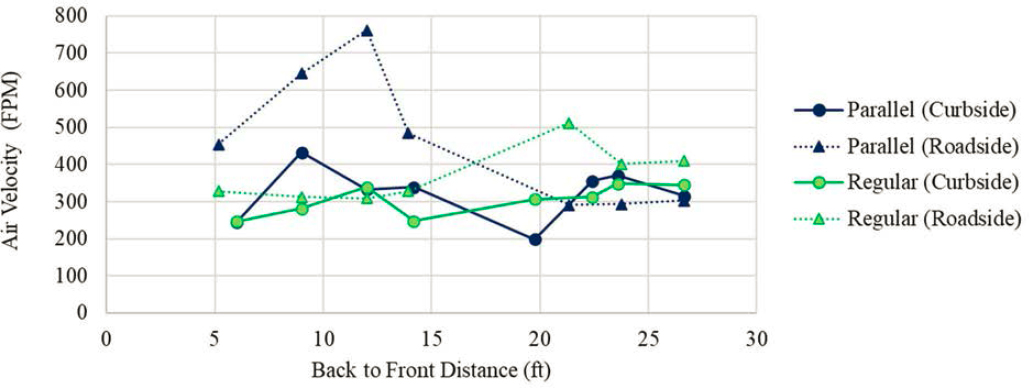
The air velocity was measured along the longitudinal lengths of the Bus A ventilation ducts for both parallel and regular systems. The bus is equipped with overhead air ducts containing two-inch outlet ventilation slots above passenger seating in the cabin. Using a TESTO 405i hot wire anemometer, air flow velocity was measured at the internal center of the duct (Figure 20). A TESTO 410i vane anemometer was used to measure air velocity at the outlets of vertical and lateral vents shown in Figure 20, respectively. The location of each measurement was approximately aligned to a corresponding floor vent in the parallel system set up. The distance was measured starting from the back wall of the cabin to the front.
Internal duct air velocities measured in the regular system are shown in Figure 21. Maximums occurred near the back of the cabin with values of 734 FPM and 468 FPM for the roadside and curbside, respectively. The largest velocities are expected near the back of the bus cabin as the regular system cycles air using blowers installed on each side of the rear panel HVAC system. Velocity trends show similar decrease throughout the length of the ducts by 26.75 FPM per foot at roadside and 24.23 FPM per foot at curbside.
Comparison to the internal duct air velocities of the parallel system is shown in Figure 22. The flow profile is expected to differ due to external blowers providing ventilation to the cabin ventilation ducts. Air velocity at vertical vents averaged 388± 150 FPM between curbside and roadside (Figure 22). The overall average air velocity at lateral vents were 323 ± 114 FPM (Figure 24). In the regular system, air velocities at vertical vents were similar between curbside and roadside with an overall average of 335 ± 67 FPM. Lateral vent velocities are also comparable with an overall average of 298±52 FPM.


Air Change per Hour: Bus B
To calculate ACH, CO2 gas was released within the bus cabin while the AC system was turned on and the AC fans set to high. The temperature within the cabin was maintained near a range of 15.5 to 17 °C.
After CO2 gas was released, it was allowed to decay while testing various ventilation conditions. Equation 1 was used as a best fit model to represent the decay within each scenario. Sensor #4 results are shown in figures throughout this section to represent a baseline example of each non-linear regression fit.
Figure 25 shows test #4 CO2 concentration inside Bus B while both doors are closed followed by opening the front door. When doors are closed, the average ACH rate is 0.67 ± 0.03 hr-1 which indicates the air volume within the bus cabin is only partly removed or replaced within an hour. When the front door is open, exchange with outside air increases as is expected and has an average of 5.33± 0.99 hr-1. Figure 26 and Figure 27 show CO2 decay where both doors are closed with the AC system set to high, but the driver fans are set to high and low, respectively. The ACH rate is higher when driver fans are set to high compared to when they are set to low as the driver fan brings fresh air from outside. Table 9 shows a summary of Bus B ACH rates per sensor for each test discussed #4-7.
A study conducted by (Shinohara et al. 2022) also used the CO2 decay method to calculate ACH rates inside a large route bus (Isuzu LV290Q1). Their stationary experiments were conducted inside a car barn to neglect the effect of outside air. The estimated ACH for this test condition with all windows and doors closed was reported to be 0.068 hr-1. This is lower compared to this test. Shinohara et al. (2022) put the bus in a barn where there is no effect of outside air whereas this test was done in an open parking lot where ambient wind conditions affect. There is also a test condition, conducted by Shinohara et al. (2022), where the bus is at 0 mph and open to the environment. Their ACH is reported to be 0.87 hr-1 with the AC on and 0.34 hr-1 with the AC off. The former is in the same order of magnitude as this test with the doors closed. The latter shows an increase compared to their enclosed method indicating that there is influence of outside air flow conditions on the bus ACH value.


Table 9: AER results in hr-1 per sensor inside Bus B.
| A/C | Hi | Hi | Hi | Hi |
|---|---|---|---|---|
| Driver fans | off | off | Hi | Lo |
| Door | Closed doors | Front door open | Closed doors | Closed doors |
| Sensor 1 | 0.69 | 5.54 | 6.30 | 4.45 |
| Sensor 2 | 0.65 | 7.16 | 6.31 | 4.70 |
| Sensor 3 | 0.61 | 4.07 | 6.17 | 4.22 |
| Sensor 4 | 0.68 | 5.40 | 5.81 | 5.11 |
| Sensor 5 | 0.71 | 6.76 | 6.43 | 4.61 |
| Sensor 6 | 0.69 | 5.49 | 6.35 | 4.56 |
| Sensor 7 | 0.64 | 4.27 | 6.40 | 4.88 |
| Sensor 8 | 0.69 | 4.93 | 6.28 | 4.76 |
| Sensor 9 | 0.64 | 4.75 | 6.44 | 4.70 |
| Sensor 10 | 0.69 | 4.98 | 6.57 | 4.43 |
| Average ± SD | 0.67 ± 0.03 | 5.33 ± 0.99 | 6.31 ± 0.21 | 4.64 ± 0.25 |
Air Change per Hour: Bus A
Non-linear regression fit models were also computed for Bus A tests #10-13. Figure 28 shows the exponential decay of CO2 measured by sensor #4 when both doors are closed. ACH rate when in this test with the AC system set to high has an average value of 1.64 ± 0.10 hr-1. This is higher when compared to Bus B by a value of 1 meaning the volume of air inside the cabin will be replaced one additional time within the same hour. This was attributed to the better door seals in Bus B reducing the space for air to enter/escape.
Figure 29 shows decay curves of a repeated doors closed scenario followed by both doors opening. The repeated test showed a higher average ACH rate of 2.54± 0.21 hr-1, however, this is attributed to outside air influence as the test conditions remained the same. Average wind speeds on this day were 8 to 10 mph. Average ACH rates are also expected to be significantly larger when both doors are open as outside air is cycled throughout the cabin at 36.48 ± 6.86 hr-1 with both doors open.
Test #12 and #13 in Figure 30 and Figure 31, respectively, incorporate the use of a Dyno blower aimed at the floor of the front door to simulate driving conditions. This is followed by turning the blower off and opening either the front or back door. ACH rates are comparable between repeated tests with simulated driving at 3.15 ± 0.36 to 3.78 ± 0.2 hr-1. Opening one of the doors does not differ greatly between the front and rear door and showed values at 12.81 ± 0.55 hr-1 and 12.23 ± 0.82 hr-1, respectively. This is a larger ACH value for the same case for Bus B bus. This was attributed to a shorter body length of Bus A facilitating better air exchange when a door is open.
Table 10 gives a summary of ACH rates determined by each sensor for tests discussed #10-13. In Shinohara et al. (2022), they tested a combination of opening windows rather than doors. However, the overall trend showed an increase in ACH as number of windows opened increased.

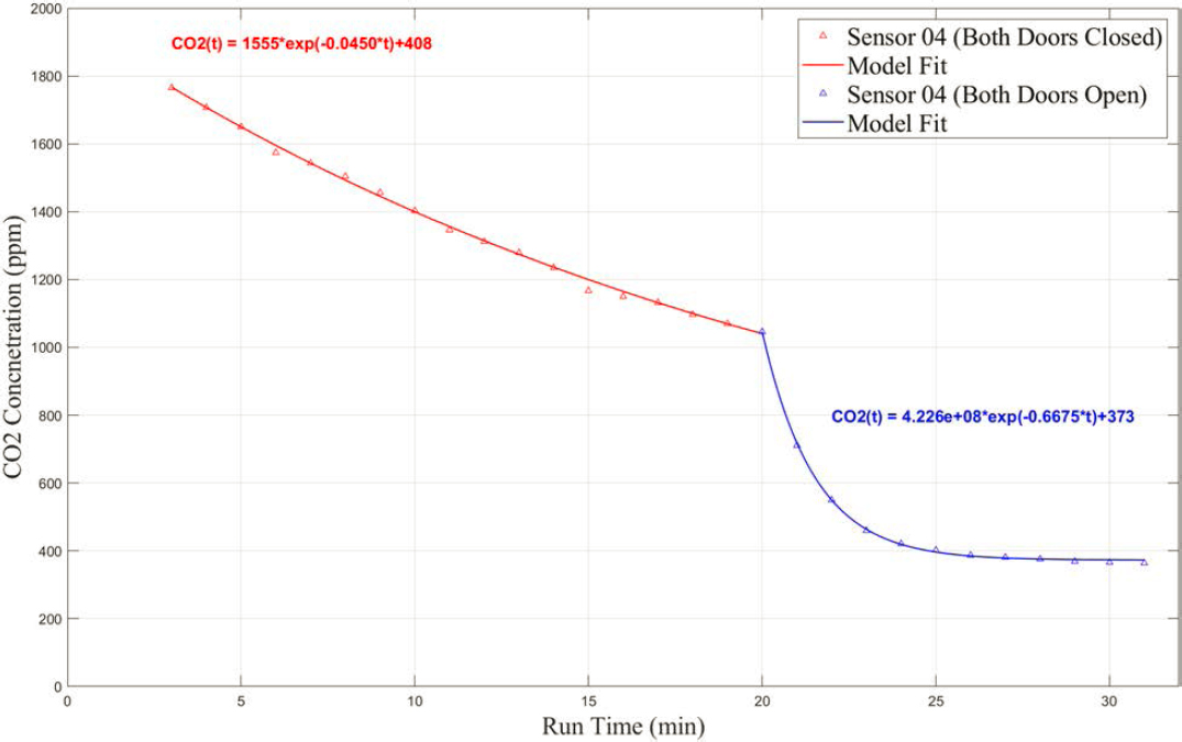
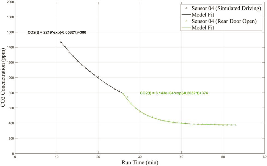

Table 10: AER results in hr-1 per sensor inside Bus A.
| A/C | Hi | Hi | Hi | Hi | Hi | Hi | Hi |
|---|---|---|---|---|---|---|---|
| Driver fans | Off | Off | Off | Off | Off | Off | Off |
| Door | Doors Closed | Doors Closed | Doors open | Simulated Driving (Dyno fan on) | Rear Door Open | Simulated Driving (Dyno fan on) | Front Door Open |
| Sensor 1 | 1.66 | 2.36 | 29.06 | 4.11 | 12.64 | 3.16 | 10.52 |
| Sensor 2 | 1.74 | 2.36 | 33.57 | 4.00 | 13.48 | 3.28 | 12.23 |
| Sensor 3 | 1.46 | 2.63 | 49.99 | 4.13 | 12.81 | 2.99 | 11.09 |
| Sensor 4 | 1.66 | 2.70 | 40.05 | 3.49 | 12.19 | 3.29 | 12.61 |
| Sensor 5 | 1.61 | 2.41 | 35.43 | 3.68 | 12.98 | 3.02 | 12.53 |
| Sensor 6 | 1.75 | 2.69 | 45.51 | 3.83 | 13.44 | 3.99 | 12.85 |
| Sensor 7 | 1.54 | 2.50 | 34.67 | 3.62 | 13.24 | 2.77 | 12.72 |
| Sensor 8 | 1.63 | 2.87 | 35.93 | 3.67 | 12.86 | 3.24 | 12.21 |
| Sensor 9 | 1.77 | 2.18 | 29.07 | 3.72 | 11.68 | 2.68 | 12.32 |
| Sensor 10 | 1.62 | 2.68 | 31.57 | 3.57 | 12.72 | 3.13 | 13.22 |
| Average ± | 1.64 ± | 2.54 ± | 36.48 ± | 3.78 ± | 12.81 ± | 3.15 ± | 12.23 ± |
| SD | 0.10 | 0.21 | 6.86 | 0.23 | 0.55 | 0.36 | 0.82 |
Air Change per Hour: On-Road Results
Non-linear regression fit models were computed for the on-road tests 2-4 and 6. Figures 32-35 show the exponential decays of CO2 measured by TSI AirAssure sensor #4 with the fitted curve. Test #2 had the aerosol generator at the front of the bus prior to driving, while for test #3 the generator was placed at the center of the bus cabin on the seat next to sensor 5. For each test, the CO2 concentration profile along with the bus driving speed profile is shown in Figure 32 and Figure 33, respectively. The average ACH rates are similar between the tests with 7.51 ± 0.52 hr-1 for test #2 and 8.46 ± 0.79 hr-1 for test #3 as expected due to similar set up.
Speed profiles show the bus cycled between 5 to 30 mph. In Shinohara et al. (2022), the test bus was driven at speeds of 10, 20, and 30 kph, which is equivalent to 6, 12, and 18 mph, respectively. Their results showed ACH values of 1.9 hr-1 for the lowest speed and up to 2.4 hr-1 for the highest speed. These values are lower than those reported in this study. There can be multiple reasons such as driving patterns, wind conditions, and bus dimensions/design for that, but overall Shinohara et al.’s (2022) results suggest their test bus was better air sealed that the test bus of this study. The higher ACH results in this study is also likely due to the difference in air pressure between the inside of the bus cabin and the outside that assists ventilation rate.
When comparing between on-road driving tests and the simulated driving using dyno fans, the ACH rates are about twice larger compared to the blower test results. This means the size of the fan did not replicate the pressure experienced by realistic driving conditions. The use of driver fans was also incorporated in test #4 (Figure 34), however, the average ACH did not vary significantly to tests without these fans. It is assumed the dynamic pressure difference allows outside air to penetrate the bus cabin regardless of the driver fan setting at this typical city driving speed.
Figure 35 shows the CO2 decay and driving speed profile for the stop-and-go test. In this study, the stop- and-go means that the bus doors were open for approximately 20 seconds at the end of each lap to simulate air exchange conditions during passenger loading and unloading with both doors open. This is similar to Shinohara et al. (2022) as their stop-and-go tests also opened the doors for 20 seconds, however, it was after moving 500m (0.3 miles) and driving 30kph (48mph). The ACH rate is 27.07 ± 0.86 hr-1 which is approximately three times more than that reported by Shinohara et al. (2022). They also tested stop-and-go
conditions with windows open and their results showed an ACH rate of 58 hr-1. Table 11 gives a summary of ACH rates per sensor for each test.
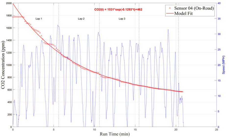
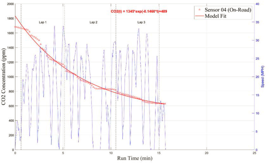


Table 11: AER results in hr-1 per sensor for on-road testing.
| A/C | Hi | Hi | Hi | |
| Driver fans | Off | Off | Hi | |
| Door | On-Road | On-Road | On-Road | Stop & Go* |
| Sensor 1 | 6.20 | 7.19 | 6.52 | 28.67 |
| Sensor 2 | 7.50 | 8.48 | 7.09 | 27.89 |
| Sensor 3 | 7.25 | 6.88 | 6.46 | 28.21 |
| Sensor 4 | 7.76 | 8.76 | 7.43 | 29.69 |
| Sensor 5 | 7.97 | 8.67 | 7.42 | 28.29 |
| Sensor 6 | 7.37 | 9.02 | 7.57 | 29.30 |
| Sensor 7 | 7.66 | 8.90 | 8.44 | 29.42 |
| Sensor 8 | 8.22 | 9.67 | 8.54 | 28.37 |
| Sensor 9 | 7.37 | 8.42 | 7.63 | 27.13 |
| Sensor 10 | 7.76 | 8.64 | 7.54 | 28.03 |
| Average ± SD | 7.51 ± 0.52 | 8.46 ± 0.79 | 7.46 ± 0.65 | 27.07 ± 0.86 |
*Stop-and-Go: Doors open at end of each loop for 20 sec at the stop position.
Particle Arrival Time
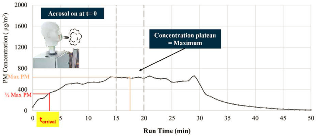
The aerosol generator was placed at different locations inside each bus cabin to determine the PM arrival time per sensor. The PM arrival time is defined as the time in minutes after the aerosol generator is powered on at which the PM concentration is measured at a value that is equal to ½ of the maximum concentration. The PM concentration plateaus after 10 to 15 minutes of the aerosol generator being on, a 5-minute average window within the plateau is used to calculate the maximum concentration per sensor (Figure 35). The ½ max PM concentration is the rise value in µg/m3 which is expected to change depending on the proximity between the generator and each sensor location. The elapsed time until the PM concentration meets or exceeds the rise value measurement is identified as the PM arrival time. This was the most reasonable choice because of the time resolution of the TSI AirAssure sensors. The sensors have a time resolution of 1 min as a default but was later updated to a time resolution of 10 second measurement. This calculation provides a measure of when the aerosol reaches each sensor throughout the cabin. To compare maximum concentrations between sensors and within each test a relative max value was obtained. This is calculated using the upper and lower quartile of each sensors’ recorded maximum and minimum PM concentration during baseline testing with the aerosol generator at the front, middle, and back. Bus B bus data used a relative min of 0 µg·m-3 and relative max of 1165 µg·m-3.
Particle Arrival: Stationary Bus
Table 12 is a summary of particle arrival times inside Bus B cabin for tests #1-#3. In baseline test #1, the AC system is off, and the aerosol generator is located at the front of the bus. Sensor #1 has the first arrival time at 2 minutes as it is the closest to the generator location. Remaining sensors have arrival times between 6-8 minutes as expected due to their increased distance away from the aerosol generator. Comparing results to baseline test #2, this time with the AC system on, sensors #2-10 have much faster arrival times of 4 and 5 minutes likely due to air flowing towards the AC inlet at the back of the cabin. In test #3, the generator is moved to the middle of the cabin next to sensor #5. Sensor #6 recorded a 1.1 relative max concentration and had the fastest arrival time showing that the flow of particles reaches across the center aisle. This behavior is expected as air is cycled towards the back panel and through the filtration medium before it reenters the cabin from the top vents. Lastly, the longest particle arrival time of 6 minutes is measured by sensor #1.
Particle Arrival: Barriers Using Conventional and Parallel Ventilation
Table 13 provides the summary of particle arrival times inside Bus A cabin for tests #4 -9 to compare the effect of barriers to baseline results. The two buses cannot be used as a direct comparison as their cabin volumes and lengths are different, therefore, a new relative minimum (1 µg·m-3) and maximum (581 µg·m-3) were calculated. With the aerosol generator placed at the front of the cabin, there is no major difference between the use of barriers in test #4 and the baseline test #9 without barriers. Particle arrival times were approximately 2 to 3 minutes throughout each sensor for both tests. This is likely due to the aerosol cloud immediately reaching the center of the aisle from the orientation of the aerosol generator (Figure 17). The baseline test #8 with the aerosol generator in the middle had a 1-minute arrival time for the sensor directly behind it. The nearby sensors at the middle and back of the cabin had faster arrival times by one minute compared to the sensors towards the front.
When barriers are present in Bus A, a faster speed of dispersion is seen for all sensors with 2-3 minute arrival times compared to 2-5 minutes without barriers. On the other hand, lower rise value concentrations are observed with barriers suggesting some particles were removed through deposition. When the aerosol generator is placed at the back of the cabin, arrival times are approximately ~3 minutes and rise value
concentrations are comparable by less than a 20 µg·m-3 difference with and without barriers. From visual inspection during testing, the aerosol plume primarily flowed near the inlet of the bus HVAC system where the MERV 13 filter is located, indicating some particles are immediately filtered from the cabin before being mixed into the cabin air.
The same baseline and barrier tests were performed using the parallel ventilation system inside the Bus A cabin. In additional testing with barriers, sections of the roof top vents were blocked off to create an air shower directly above the floor vent openings from the parallel system. Table 14 summarizes particle arrival times for these tests #10-#18 using higher resolution data of 10 second intervals. Additionally, to evaluate inner window seat particle exposures, sensors #11-18 were paired next to the original 10 sensor placement. The baseline test #10 with the aerosol generator at the front showed the highest relative max concentration of 1.5 and particle arrival time of 0.3 min (18 seconds) at sensor #2. This is followed by sensor #4, which is located immediately behind, having the same particle arrival time and a lower relative max concentration of 1.0. Relative max concentrations are lower for nearby sensors, 0.8 for sensor #12 and 0.6 for sensor #1.
Although arrival times throughout the cabin are still below 2-3 minutes, the concentrations experienced from the sensors towards the rear of the cabin are significantly lower with values of 0.1-0.4, than the regular system baseline test with values of 0.6-1.0. When barriers are installed, test #13 showed no major difference between PM concentrations to the baseline parallel test, yet arrival times were improved by an average of 0.4 minutes. This means barriers delay particle arrival times only by a few seconds when the source is at the front of the bus. Test #16 used an air shower method discussed earlier in conjunction to installed barriers. This combination showed the best improvement for reducing concentrations with relative maximum values below 0.5 for sensors #2-18. The concentration was highest only between the first seats near the aerosol generator. Arrival times gradually increased from 0.8 up to 2.3 minutes from aisle seat sensors #1 to #10 and 0.7 to 3.5 minutes from window seat sensors #11-#18. When the aerosol generator is moved to the middle of the cabin next to sensor #5, the baseline test #11 indicates the highest concentration occurs near sensors #3 and #13 at values of 0.9 and 1.6 respectively. The seat at the aerosol location to the seats where sensors #3 and #13 are located, are only separated by the entry space from the bus side door. This indicates the aerosol plume can reach a distance larger than the seats directly in front of it with the parallel system whereas the regular system affects the seat directly behind the source. Barriers help mitigate this issue shown by test #14, where sensors #3 and #13 remain below a relative max concentration of 0.2 and Sensor #5 experiences the highest concentration of 1.4 with only barriers and 0.9 with both barriers and air shower. Longer arrival times are seen when using the air shower method with 2.8 minutes at the front of the cabin and 3.2 minutes at the back of the cabin. Lastly, when the aerosol generator is placed at the back of the bus cabin, the baseline test #12, the barrier test #15, and the air shower test #18 showed no major difference in maximum concentration values. However, in comparison to the conventional ventilation system, relative maximum concentrations were still lower at locations near the middle and front of the bus. When analyzing particle arrival times, the parallel system showed faster arrival times overall with a range from 0.5 min at the back and 3.5 near the front.
Collectively, there is a tradeoff between arrival times and maximum concentrations throughout the bus cabin depending on the location, ventilation type, and use of barriers. The regular system showed longer particle arrival times by 1 to 2 minutes compared to the parallel system but had larger exposures with relative aerosol concentrations above 0.5 (~290 µg*m-3) throughout the cabin. The use of barriers in the regular system primarily impacted results when the aerosol generator was in the middle. This caused faster arrival times by 2 minutes but had lower concentrations overall. Installing barriers in the parallel system delayed arrival times by 0.4 minutes but no difference is seen in relative maximum concentrations from baseline.
Particle Arrival: Air Shower Parallel Ventilation System
The combination of an air shower with barriers is an optimum solution as the exposure concentrations were the lowest overall with maximum concentrations of 0.8-1.1 (~ 465 – 639 µg*m-3) directly next to the
aerosol generator and concentrations less than 0.5 (~290 µg*m-3) everywhere else in the bus cabin. This combination creates an effective partition throughout the cabin to keep aerosol plume concentrations within the immediate source area. This also impacts delay in arrival times throughout the bus. When the aerosol generator is at the front arrival times ranged from 0.8 minutes at the source to 2.3 minutes away from the source. If the aerosol generator is placed at the back, this range increases from 0.5 to 3.3 minutes. When placed in the middle, arrival times take 2.5 at the front and 3.2 at the back of the cabin.
Table 12: Particle arrival times per sensor inside Bus B with regular HVAC bus cabin for tests 1-3.
| Test #1 Baseline, Front Seat Aerosol Location | ||||||||||
| AC | Off | |||||||||
| Sensor # | 1 | 2 | 3 | 4 | 5 | 6 | 7 | 8 | 9 | 10 |
| Relative Max Value* (µg*m-3/µg*m-3) | 1.0 | 1.1 | 0.4 | 0.4 | 0.5 | 0.5 | 0.3 | 0.3 | 0.4 | 0.3 |
| Rise Value (µg/m-3) | 603 | 646 | 226 | 224 | 313 | 280 | 176 | 188 | 218 | 161 |
| Arrival Time (min) | 2 | 2 | 7 | 6 | 7 | 6 | 8 | 8 | 7 | 8 |
| Test #2 Baseline, Front Seat Aerosol Location | ||||||||||
| AC | Hi | |||||||||
| Sensor # | 1 | 2 | 3 | 4 | 5 | 6 | 7 | 8 | 9 | 10 |
| Relative Max Value* (µg*m-3/µg*m-3) | 0.9 | 0.6 | 0.4 | 0.5 | 0.7 | 0.6 | 0.4 | 0.6 | 0.4 | 0.3 |
| Rise Value (µg/m-3) | 531 | 355 | 236 | 318 | 429 | 350 | 230 | 356 | 261 | 199 |
| Arrival Time (min) | 2 | 4 | 4 | 3 | 4 | 4 | 4 | 4 | 4 | 5 |
| Test #3 Baseline, Middle Seat Aerosol Location | ||||||||||
| AC | Hi | |||||||||
| Sensor # | 1 | 2 | 3 | 4 | 5 | 6 | 7 | 8 | 9 | 10 |
| Relative Max Value* (µg*m-3/µg*m-3) | 0.4 | 0.3 | 0.2 | 0.3 | 0.6 | 1.1 | 0.4 | 0.7 | 0.4 | 0.4 |
| Rise Value (µg/m-3) | 220 | 204 | 132 | 183 | 324 | 620 | 211 | 410 | 234 | 221 |
| Arrival Time (min) | 6 | 5 | 5 | 5 | 5 | 2 | 4 | 3 | 4 | 3 |
* Relative min: 0 µg*m-3 & Relative max: 1165 µg*m-3
Table 13: Particle arrival time per sensor with conventional ventilation system for Bus A tests 4-9.
| Test #4 Barriers Installed, Front Seat Aerosol Location | ||||||||||
| AC | Hi | |||||||||
| Sensor # | 1 | 2 | 3 | 4 | 5 | 6 | 7 | 8 | 9 | 10 |
| Relative Max Value† (µg*m-3/µg*m-3) | 1.1 | 0.9 | 0.5 | 0.6 | 0.9 | 0.6 | 0.4 | 0.4 | 0.5 | 0.4 |
| Rise Value (µg/m-3) | 314 | 249 | 136 | 183 | 250 | 188 | 126 | 122 | 145 | 118 |
| Arrival Time (min) | 2 | 2 | 2 | 2 | 2 | 3 | 2 | 3 | 2 | 3 |
| Test #5 Barriers Installed, Middle Seat Aerosol Location | ||||||||||
| AC | Hi | |||||||||
| Sensor # | 1 | 2 | 3 | 4 | 5 | 6 | 7 | 8 | 9 | 10 |
| Relative Max Value† (µg*m-3/µg*m-3) | 0.6 | 0.5 | 0.3 | 0.4 | 0.8 | 0.7 | 0.5 | 0.6 | 0.5 | 0.5 |
| Rise Value (µg/m-3) | 163 | 141 | 79 | 122 | 239 | 200 | 144 | 173 | 143 | 157 |
| Arrival Time (min) | 3 | 3 | 3 | 3 | 2 | 2 | 3 | 2 | 2 | 2 |
| Test #6 Barriers Installed, Back Seat Aerosol Location | ||||||||||
| AC | Hi | |||||||||
| Sensor # | 1 | 2 | 3 | 4 | 5 | 6 | 7 | 8 | 9 | 10 |
| Relative Max Value† (µg*m-3/µg*m-3) | 0.6 | 0.5 | 0.3 | 0.4 | 0.7 | 0.6 | 0.4 | 0.4 | 0.5 | 0.4 |
| Rise Value (µg/m-3) | 180 | 153 | 91 | 124 | 203 | 174 | 126 | 124 | 137 | 116 |
| Arrival Time (min) | 3 | 3 | 3 | 3 | 3 | 3 | 3 | 3 | 3 | 3 |
| Test #7 No Barriers, Back Seat Aerosol Location | ||||||||||
| AC | Hi | |||||||||
| Sensor # | 1 | 2 | 3 | 4 | 5 | 6 | 7 | 8 | 9 | 10 |
| Relative Max Value† (µg*m-3/µg*m-3) | 0.6 | 0.5 | 0.4 | 0.5 | 0.7 | 0.6 | 0.4 | 0.6 | 0.5 | 0.4 |
| Rise Value (µg/m-3) | 175 | 160 | 120 | 140 | 215 | 189 | 124 | 177 | 136 | 118 |
| Arrival Time (min) | 4 | 3 | 4 | 3 | 4 | 3 | 4 | 4 | 4 | 4 |
| Test #8 No Barriers, Middle Seat Aerosol Location | ||||||||||
| AC | Hi | |||||||||
| Sensor # | 1 | 2 | 3 | 4 | 5 | 6 | 7 | 8 | 9 | 10 |
| Relative Max Value† (µg*m-3/µg*m-3) | 0.8 | 0.6 | 0.6 | 0.6 | 1.1 | 0.8 | 0.9 | 0.8 | 0.9 | 0.6 |
| Rise Value (µg/m-3) | 236 | 181 | 177 | 173 | 305 | 230 | 248 | 240 | 252 | 162 |
| Arrival Time (min) | 5 | 3 | 5 | 4 | 3 | 3 | 1 | 3 | 2 | 2 |
| Test #9 No Barriers, Front Seat Aerosol Location | ||||||||||
| AC | Hi | |||||||||
| Sensor # | 1 | 2 | 3 | 4 | 5 | 6 | 7 | 8 | 9 | 10 |
| Relative Max Value† (µg*m-3/µg*m-3) | 1.0 | 0.9 | 0.7 | 0.8 | 1.0 | 1.0 | 0.6 | 0.9 | 0.7 | 0.6 |
| Rise Value (µg/m-3) | 290 | 249 | 199 | 225 | 302 | 304 | 177 | 272 | 204 | 178 |
| Arrival Time (min) | 2 | 2 | 3 | 2 | 3 | 3 | 3 | 2 | 3 | 3 |
† Relative min: 1 µg*m-3 & Relative max: 581 µg*m-3
Table 14: Particle arrival time per sensor with parallel system for Bus A tests 10-18.
| Test #10 Parallel Baseline, Front Seat Aerosol Location | ||||||||||
| AC | Hi | |||||||||
| Sensor # | 1 | 2 | 3 | 4 | 5 | 6 | 7 | 8 | 9 | 10 |
| Relative Max Value (µg*m-3/µg*m-3) | 0.6 | 1.5 | 0.2 | 1.0 | 0.3 | 0.4 | 0.2 | 0.2 | 0.2 | 0.1 |
| Rise Value (µg/m-3) | 171 | 425 | 54 | 293 | 82 | 105 | 56 | 67 | 45 | 32 |
| Arrival Time (min) | 0.7 | 0.3 | 1.7 | 0.3 | 1.3 | 1.0 | 1.3 | 1.0 | 2.0 | 2.0 |
| Sensor # | 11 | 12 | 13 | 14 | 15 | 16 | 17 | 18 | ||
| Relative Max Value (µg*m-3/µg*m-3) | 0.3 | 0.8 | 0.2 | 1.1 | 0.2 | 0.4 | 0.3 | 0.2 | ||
| Rise Value (µg/m-3) | 87 | 218 | 67 | 322 | 50 | 110 | 76 | 54 | ||
| Arrival Time (min) | 1.5 | 1.5 | 2.0 | 0.7 | 1.7 | 1.2 | 0.8 | 3.0 | ||
| Test #11 Parallel Baseline, Middle Seat Aerosol Location | ||||||||||
| AC | Hi | |||||||||
| Sensor # | 1 | 2 | 3 | 4 | 5 | 6 | 7 | 8 | 9 | 10 |
| Relative Max Value (µg*m-3/µg*m-3) | 0.5 | 0.3 | 0.9 | 0.3 | 0.4 | 0.4 | 0.3 | 0.3 | 0.2 | 0.2 |
| Rise Value (µg/m-3) | 140 | 90 | 266 | 98 | 125 | 119 | 82 | 95 | 73 | 50 |
| Arrival Time (min) | 1.2 | 1.7 | 0.3 | 0.8 | 1.2 | 1.0 | 1.2 | 1.2 | 1.5 | 1.8 |
| Sensor # | 11 | 12 | 13 | 14 | 15 | 16 | 17 | 18 | ||
| Relative Max Value (µg*m-3/µg*m-3) | 0.7 | 0.3 | 1.6 | 0.4 | 0.3 | 0.5 | 0.4 | 0.3 | ||
| Rise Value (µg/m-3) | 200 | 75 | 477 | 127 | 82 | 132 | 113 | 81 | ||
| Arrival Time (min) | 1.7 | 2.0 | 0.7 | 1.2 | 1.3 | 1.3 | 0.8 | 2.7 | ||
| Test #12 Parallel Baseline, Back Seat Aerosol Location | ||||||||||
| AC | Hi | |||||||||
| Sensor # | 1 | 2 | 3 | 4 | 5 | 6 | 7 | 8 | 9 | 10 |
| Relative Max Value (µg*m-3/µg*m-3) | 0.2 | 0.2 | 0.3 | 0.1 | 0.5 | 0.3 | 0.3 | 0.4 | 1.2 | 0.8 |
| Rise Value (µg/m-3) | 56 | 45 | 81 | 38 | 147 | 73 | 84 | 115 | 356 | 231 |
| Arrival Time (min) | 2.5 | 2.0 | 1.5 | 2.0 | 1.3 | 1.7 | 1.7 | 1.2 | 0.7 | 1.0 |
| Sensor # | 11 | 12 | 13 | 14 | 15 | 16 | 17 | 18 | ||
| Relative Max Value (µg*m-3/µg*m-3) | 0.2 | 0.1 | 0.4 | 0.2 | 0.4 | 0.3 | 0.4 | 0.4 | ||
| Rise Value (µg/m-3) | 59 | 39 | 111 | 47 | 107 | 83 | 123 | 126 | ||
| Arrival Time (min) | 1.5 | 2.7 | 1.8 | 2.7 | 1.5 | 2.0 | 1.0 | 2.3 | ||
| Test #13 Parallel System with Barriers Installed, Front Seat Aerosol Location | ||||||||||
| AC | ||||||||||
| Sensor # | 1 | 2 | 3 | 4 | 5 | 6 | 7 | 8 | 9 | 10 |
| Relative Max Value (µg*m-3/µg*m-3) | 0.5 | 1.2 | 0.4 | 0.6 | 0.6 | 0.3 | 0.2 | 0.2 | 0.2 | 0.1 |
| Rise Value (µg/m-3) | 147 | 336 | 117 | 179 | 176 | 99 | 57 | 60 | 54 | 40 |
| Arrival Time (min) | 1.2 | 0.3 | 1.5 | 0.8 | 1.7 | 1.8 | 2.0 | 1.8 | 2.3 | 2.5 |
| Sensor # | 11 | 12 | 13 | 14 | 15 | 16 | 17 | 18 | ||
| Relative Max Value (µg*m-3/µg*m-3) | 0.4 | 0.8 | 0.5 | 0.6 | 0.4 | 0.3 | 0.2 | 0.2 | ||
| Rise Value (µg/m-3) | 106 | 220 | 150 | 173 | 118 | 87 | 69 | 63 | ||
| Arrival Time (min) | 1.3 | 0.7 | 1.7 | 1.3 | 1.8 | 2.2 | 1.7 | 2.8 | ||
| Test #14 Parallel System with Barriers Installed, Middle Seat Aerosol Location | ||||||||||
| AC | ||||||||||
| Sensor # | 1 | 2 | 3 | 4 | 5 | 6 | 7 | 8 | 9 | 10 |
| Relative Max Value (µg*m-3/µg*m-3) | 0.2 | 0.2 | 0.1 | 0.3 | 1.4 | 0.6 | 0.3 | 0.3 | 0.3 | 0.2 |
| Rise Value (µg/m-3) | 56 | 58 | 43 | 95 | 401 | 174 | 82 | 99 | 83 | 62 |
| Arrival Time (min) | 1.3 | 1.3 | 0.8 | 1.3 | 0.0 | 0.0 | 0.5 | 0.2 | 0.8 | 0.8 |
| Sensor # | 11 | 12 | 13 | 14 | 15 | 16 | 17 | 18 | ||
| Relative Max Value (µg*m-3/µg*m-3) | 0.2 | 0.2 | 0.2 | 0.3 | 0.4 | 0.4 | 0.4 | 0.3 | ||
| Rise Value (µg/m-3) | 45 | 59 | 66 | 83 | 115 | 113 | 106 | 95 | ||
| Arrival Time (min) | 1.8 | 1.5 | 1.0 | 1.5 | 0.2 | 0.7 | 0.3 | 1.3 | ||
| Test #15 Parallel System with Barriers Installed, Back Seat Aerosol Location | ||||||||||
| AC | ||||||||||
| Sensor # | 1 | 2 | 3 | 4 | 5 | 6 | 7 | 8 | 9 | 10 |
| Relative Max Value (µg*m-3/µg*m-3) | 0.1 | 0.1 | 0.1 | 0.1 | 0.3 | 0.2 | 0.3 | 0.3 | 0.4 | 0.6 |
| Rise Value (µg/m-3) | 27 | 28 | 25 | 31 | 78 | 70 | 87 | 87 | 113 | 162 |
| Arrival Time (min) | 2.5 | 2.3 | 1.8 | 2.3 | 1.7 | 1.7 | 1.3 | 1.2 | 1.5 | 0.3 |
| Sensor # | 11 | 12 | 13 | 14 | 15 | 16 | 17 | 18 | ||
| Relative Max Value (µg*m-3/µg*m-3) | 0.1 | 0.1 | 0.1 | 0.1 | 0.2 | 0.2 | 0.4 | 0.2 | ||
| Rise Value (µg/m-3) | 22 | 25 | 38 | 39 | 62 | 64 | 118 | 65 | ||
| Arrival Time (min) | 2.5 | 2.7 | 2.0 | 2.3 | 1.7 | 2.0 | 1.2 | 2.3 | ||
| Test #16 Parallel System With Barriers Installed And Taped Vents, Front Seat Aerosol Location | ||||||||||
| AC | ||||||||||
| Sensor # | 1 | 2 | 3 | 4 | 5 | 6 | 7 | 8 | 9 | 10 |
| Relative Max Value (µg*m-3/µg*m-3) | 0.8 | 0.4 | 0.4 | 0.4 | 0.4 | 0.2 | 0.1 | 0.1 | 0.1 | 0.1 |
| Rise Value (µg/m-3) | 246 | 131 | 120 | 113 | 118 | 70 | 22 | 22 | 21 | 17 |
| Arrival Time (min) | 0.8 | 0.8 | 1.0 | 1.2 | 2.0 | 2.0 | 2.5 | 2.8 | 2.3 | 2.3 |
| Sensor # | 11 | 12 | 13 | 14 | 15 | 16 | 17 | 18 | ||
| Relative Max Value (µg*m-3/µg*m-3) | 0.8 | 0.3 | 0.5 | 0.5 | 0.3 | 0.2 | 0.1 | 0.1 | ||
| Rise Value (µg/m-3) | 233 | 101 | 152 | 159 | 78 | 68 | 29 | 23 | ||
| Arrival Time (min) | 0.7 | 1.5 | 1.3 | 1.7 | 2.3 | 2.2 | 2.2 | 3.5 | ||
| Test #17 Parallel System With Barriers Installed And Taped Vents, Middle Seat Aerosol Location | ||||||||||
| AC | ||||||||||
| Sensor # | 1 | 2 | 3 | 4 | 5 | 6 | 7 | 8 | 9 | 10 |
| Relative Max Value (µg*m-3/µg*m-3) | 0.1 | 0.1 | 0.3 | 0.2 | 0.9 | 1.2 | 0.2 | 0.2 | 0.1 | 0.1 |
| Rise Value (µg/m-3) | 41 | 40 | 81 | 67 | 268 | 339 | 49 | 52 | 39 | 30 |
| Arrival Time (min) | 2.8 | 2.5 | 1.5 | 2.3 | 1.0 | 1.3 | 2.3 | 2.0 | 2.3 | 2.3 |
| Sensor # | 11 | 12 | 13 | 14 | 15 | 16 | 17 | 18 | ||
| Relative Max Value (µg*m-3/µg*m-3) | 0.1 | 0.1 | 0.4 | 0.2 | 0.6 | 1.1 | 0.2 | 0.2 | ||
| Rise Value (µg/m-3) | 31 | 31 | 127 | 72 | 178 | 329 | 57 | 50 | ||
| Arrival Time (min) | 2.5 | 3.3 | 1.8 | 2.8 | 1.2 | 1.5 | 1.8 | 3.2 | ||
| Test #18 Parallel System With Barriers Installed And Taped Vents, Back Seat Aerosol Location | ||||||||||
| AC | ||||||||||
| Sensor # | 1 | 2 | 3 | 4 | 5 | 6 | 7 | 8 | 9 | 10 |
| Relative Max Value (µg*m-3/µg*m-3) | 0.1 | 0.1 | 0.0 | 0.1 | 0.2 | 0.2 | 0.5 | 0.5 | 1.0 | 1.4 |
| Rise Value (µg/m-3) | 16 | 15 | 13 | 16 | 65 | 58 | 159 | 159 | 295 | 395 |
| Arrival Time (min) | 3.3 | 3.0 | 2.7 | 3.0 | 2.2 | 2.0 | 0.8 | 0.8 | 0.8 | 0.5 |
| Sensor # | 11 | 12 | 13 | 14 | 15 | 16 | 17 | 18 | ||
| Relative Max Value (µg*m-3/µg*m-3) | 0.0 | 0.0 | 0.1 | 0.1 | 0.2 | 0.2 | 0.6 | 0.6 | ||
| Rise Value (µg/m-3) | 13 | 14 | 21 | 20 | 51 | 62 | 184 | 170 | ||
| Arrival Time (min) | 3.0 | 3.3 | 2.7 | 3.5 | 2.2 | 2.2 | 0.8 | 2.0 | ||
PM Removal Rate (eACH)
Particle removal rates can be expressed through an eACH rate from the exponential PM decay rate after the aerosol generator is turned off. The tests were conducted by placing the aerosol generator at different locations inside the bus cabin and allowing for PM 2.5 concentrations to stabilize before turning off the generator. Once the generator is off, the concentration begins to decay due to the combination of particles being removed from the bus filtration system and ventilation from outdoor air but also from particle deposition to the wall.
PM Removal: Stationary Bus A and Bus B
Figures 36-38 show the PM concentration decay rates measured by the baseline sensor #4 in comparison to the average value of all ten sensors in stationary tests #1-3 in Table 15. The eACH rate is equivalent to the exponential time coefficient as expressed in Equation 2 multiplied by 60 to convert to a per hour equivalent. Bus B test #1 is a baseline experiment with the bus engine and HVAC system off, and the aerosol generator located in the front seat of the cabin. The eACH rate average for all sensors is 4.61 ± 0.38 hr -1. A comparison baseline test #2 with the AC system on is shown in Figure 37. The eACH rate increases to a value of 9.46 ± 0.20 hr-1 showing the effect of AC system (including the duct, blower, and in-use MERV 13 filter) in removing particles.
Figure 38 shows test #3 with exponential decay while the AC system is on and the aerosol generator is moved to the middle of the bus cabin. The eACH rate for test #3 is 10.85 ± 0.21 hr-1 which is slightly higher than test #2. In other words, if a passenger sitting in a middle seat coughs, it can be removed faster compared to a cough from a passenger sitting in a front seat. This makes sense considering the bus HVAC system is designed to have a longitudinal flow from the front to the back where the MERV 13 filter and recirculating blower fan is placed.
Additional stationary tests using Bus A cabin in Table 16 showed that the baseline eACH average rate of 9.17 ±0.19 hr-1 with the aerosol generator in the front is comparable to the baseline test using Bus B
cabin. As shown previously in ACH test, Bus A had a leakier cabin air system than Bus B. This means it is bad because more air pollutants can penetrate into leakier cabin and passengers are exposed to higher concentrations of air pollutants. However, it is a good thing to lower airborne virus concentrations in the bus cabin and a leakier cabin means more dilution effect resulting in lower airborne virus concentrations.
PM Removal: Barriers
The effect of barriers is observed by placing the aerosol generator in the front, middle, and back of the bus cabin and produced eACH rates of 11.82 ±0.33 hr-1, 11.41 ±0.20 hr-1, and 12.74 ±0.27 hr-1. This shows a small increase from baseline results likely due to the ejection distance of the aerosolized salt plume. When the aerosol generator is placed at the front of the bus, it faces perpendicular to the aisle. The plume was observed to reach the aisle centerline therefore the barriers do not block the distribution of the aerosol.
PM Removal: Stand Alone Air Cleaners
This is also observed in tests #4-9 in Table 16. The eACH rate does not differ when barriers are used in conjunction with HEPA filters to rates when using standalone HEPA filters. The rate is approximately 30 hr-1 with standard deviations below 1.08 hr-1 when these on-board air cleaners are used, and it is comparable to the rate observed during on-road testing using Bus B.
Figure 39 and Figure 41 show exponential decays resulting from the use of two Honeywell HEPA air purifiers (rated 320 cfm each) in tandem with the bus AC system. The eACH rates significantly increased to values of 22.97 ± 0.38 hr-1 and 24.69 ± 0.84 hr-1 with the aerosol generator is located at the front and middle of the bus cabin, respectively. This shows that a very effective remedy to remove viruses in air is to install standalone HEPA air purifiers along with the equipped HVAC system. Figure 40 and Figure 42 provide a repeated baseline comparison to the prior tests, respectively. This is also explained for the increased eACH rate using two Honeywell HEPA air purifiers in tandem with the bus AC system from 22.97 ± 0.38 hr-1 when the bus is stationary to a rate of 31.76±0.44 hr-1 when the bus is on the road.
PM Removal: Parallel Ventilation and Air Shower System
The effectiveness of ventilation design changes using a parallel airflow system on eACH rates is summarized in Table 17 for tests #10-18 using a baseline test, installed barriers, and an air shower technique. The baseline test uses external blowers which supply air to the top vents in while removing air from floor vents throughout the cabin creating a parallel (or vertical) air flow. Barriers are placed in exact locations as the conventional ventilation system test. The air shower tests use only open slots in the top vents which are directly above the floor vents while blocking remaining air slots, creating an air shower technique. The parallel ventilation system shows larger eACH rates by at least 4.6 times in baseline tests and ~3.2 times for barrier test conditions in comparison to the conventional ventilation system (both stationary and on-road tests). This suggests much more effective removal of airborne viruses using the parallel ventilation system. The baseline test with the aerosol generator in the front, middle, and back cabin location had rates of 41.99 ± 5.40 hr-1, 44.21 ± 2.30 hr-1, and 42.40 ± 6.49 hr-1. The use of barriers and the air shower technique resulted in similar eACH rate averages for each placement of the aerosol generator. However, there are large deviations between sensor eACH rates throughout the bus that are dependent on the proximity to the aerosol generator position.
PM Removal: On-Road Tests
A summary of eACH rates from on-road testing is shown in Table 18. On-road eACH rates were shown to be higher than stationary tests with the AC on condition with 12.46±0.09 hr-1 and 12.76±0.09 hr-1 when the aerosol generator was placed at the front and middle, respectively. This is indicative of a dilution effect with more outside air penetrating into the bus cabin due to dynamic pressure difference while the bus is in motion. (Note: Outside air has lower concentrations of virus-like particles compared to inside air. It will be
an opposite story if it is about air pollutant concentrations from exhaust and non-exhaust of vehicles.) When driver fans were turned on, there was no significant increase in eACH rate and is reported to be 12.47±0.12 hr-1. This unchanged rate is speculated to be a result of the bus cabin leakage during driving to be more effective than when driver fans are on or off.


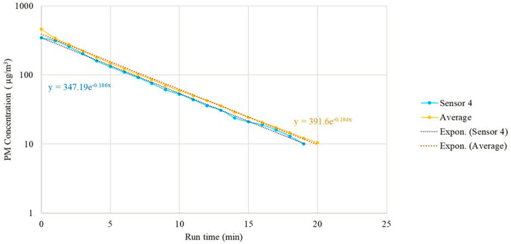


Table 15: eACH for Bus B tests 1-3 & 9-12.
| Bus B | |||||||
| Experimental Condition | Baseline | Baseline | Baseline | HEPA | Baseline Repeat | HEPA | Baseline Repeat |
| AC Fan | Off | Hi | Hi | Hi | Hi | Hi | Hi |
| Driver Fan | - | - | - | - | - | - | - |
| Aerosol Generator | Front | Front | Middle | Front | Front | Middle | Middle |
| Location | Seat | Seat | Seat | Seat | Seat | Seat | Seat |
| PM Removal Rates, eACH (hr-1) | |||||||
| Sensor 1 | 5.16 | 9.54 | 10.92 | 22.20 | 7.80 | 23.34 | 8.22 |
| Sensor 2 | 5.22 | 9.48 | 11.10 | 22.92 | 7.74 | 23.28 | 8.22 |
| Sensor 3 | 4.80 | 9.00 | 10.68 | 22.92 | 7.80 | 24.78 | 8.34 |
| Sensor 4 | 4.56 | 9.66 | 11.16 | 22.68 | 7.92 | 25.26 | 8.52 |
| Sensor 5 | 4.62 | 9.48 | 11.04 | 22.98 | 7.92 | 24.66 | 8.16 |
| Sensor 6 | 4.56 | 9.60 | 10.92 | 22.98 | 7.80 | 25.32 | 8.1 |
| Sensor 7 | 4.56 | 9.30 | 10.62 | 23.28 | 7.74 | 24.12 | 8.34 |
| Sensor 8 | 4.32 | 9.66 | 10.62 | 22.86 | 7.68 | 25.44 | 7.92 |
| Sensor 9 | 4.14 | 9.42 | 10.80 | 23.58 | 7.80 | 25.32 | 8.04 |
| Sensor 10 | 4.14 | 9.42 | 10.62 | 23.34 | 7.62 | 25.38 | 8.4 |
| Average ± SD | 4.61± 0.37 | 9.46 ± 0.20 | 10.85 ± 0.21 | 22.97 ± 0.38 | 7.78 ± 0.09 | 24.69 ± 0.84 | 8.23 ± 0.18 |
Table 16: eACH for Bus A bus tests 1-9 & 22.
| Bus A | Regular System | Regular System | Regular System | Regular System | Regular System | Regular System | Regular System | Regular System | Regular System | Regular System |
|---|---|---|---|---|---|---|---|---|---|---|
| Experimental Condition | Baseline | Barriers | Barriers | Barriers | HEPA+ Barriers | HEPA + Barriers | HEPA + Barriers | HEPA only | HEPA only | HEPA only |
| AC Fan | Hi | Hi | Hi | Hi | Hi | Hi | Hi | Hi | Hi | Hi |
| Driver Fan | - | - | - | - | - | - | - | - | - | - |
| Aerosol Generator Location | Front | Front | Middle | Back | Front | Middle | Back | Back | Middle | Front |
| PM Removal Rates, eACH (hr-1) | ||||||||||
| Sensor 1 | 9.12 | 11.88 | 11.34 | 12.78 | 29.70 | 28.92 | 28.20 | 29.58 | 30.06 | 30.90 |
| Sensor 2 | 9.18 | 11.88 | 11.7 | 12.6 | 30.66 | 29.04 | 27.90 | 30.36 | 30.18 | 30.66 |
| Sensor 3 | 9.54 | 12.3 | 11.7 | 13.44 | 29.52 | 30.54 | 27.90 | 29.16 | 30.18 | 30.72 |
| Sensor 4 | 9.18 | 12.42 | 11.7 | 12.84 | 30.12 | 28.50 | 26.34 | 30.54 | 30.84 | 30.96 |
| Sensor 5 | 9.18 | 11.76 | 11.28 | 12.72 | 29.88 | 30.18 | 28.86 | 30.18 | 30.78 | 31.32 |
| Sensor 6 | 9.00 | 11.46 | 11.22 | 12.36 | 31.20 | 31.44 | 30.24 | 31.20 | 29.88 | 31.44 |
| Sensor 7 | 9.36 | 11.94 | 11.22 | 12.84 | 31.74 | 30.18 | 29.28 | 30.60 | 31.80 | 31.62 |
| Sensor 8 | 8.82 | 11.34 | 11.34 | 12.48 | 30.72 | 32.04 | 28.98 | 30.06 | 30.42 | 32.04 |
| Sensor 9 | 9.06 | 11.7 | 11.22 | 12.66 | 30.30 | 30.18 | 29.16 | 29.82 | 31.74 | 31.68 |
| Sensor 10 | 9.30 | 11.52 | 11.34 | 12.72 | 31.50 | 31.08 | 29.10 | 31.44 | 30.96 | 32.16 |
| Average ± SD | 9.17 ±0.19 | 11.82 ±0.33 | 11.41 ±0.20 | 12.74 ±0.27 | 30.53 ±0.73 | 30.21 ±1.08 | 28.60 ±1.01 | 30.29 ±0.66 | 30.68 ±0.64 | 31.35 ±0.51 |
Table 17: Equivalent Air Changes per Hour (eACH) for Bus A bus tests 10-18.
| Bus A | Parallel | Parallel | Parallel | Parallel | Parallel | Parallel | Parallel | Parallel | Parallel |
|---|---|---|---|---|---|---|---|---|---|
| Experimental Condition | Baseline | Baseline | Baseline | Barriers | Barriers | Barriers | Air Shower | Air Shower | Air Shower |
| AC Fan | Hi | Hi | Hi | Hi | Hi | Hi | Hi | Hi | Hi |
| Driver Fan | - | - | - | - | - | - | - | - | - |
| Aerosol Generator Location | Front | Middle | Back | Front | Middle | Back | Front | Middle | Back |
| PM Removal Rates, eACH (hr-1) | |||||||||
| Sensor 1 | 45.84 | 42.12 | 35.04 | 36.60 | 33.60 | 24.78 | 33.36 | 32.22 | 20.34 |
| Sensor 2 | 49.5 | 44.04 | 34.08 | 37.26 | 34.56 | 26.46 | 36.24 | 35.28 | 19.08 |
| Sensor 3 | 40.56 | 48 | 43.02 | 36.90 | 38.52 | 31.14 | 37.02 | 39.48 | 19.02 |
| Sensor 4 | 49.44 | 45.12 | 31.50 | 39.90 | 37.56 | 32.52 | 38.52 | 38.82 | 22.92 |
| Sensor 5 | 42.3 | 45.66 | 44.70 | 38.22 | 44.94 | 37.32 | 36.24 | 40.62 | 32.58 |
| Sensor 6 | 44.82 | 46.5 | 41.10 | 36.48 | 45.06 | 38.76 | 36.54 | 42.42 | 35.58 |
| Sensor 7 | 40.32 | 44.52 | 45.96 | 36.90 | 44.28 | 45.84 | 35.94 | 35.7 | 51.48 |
| Sensor 8 | 39.54 | 44.34 | 47.70 | 32.88 | 43.62 | 42.18 | 33.66 | 35.7 | 51.48 |
| Sensor 9 | 36.24 | 42.3 | 51.06 | 34.62 | 43.56 | 44.46 | 37.38 | 33.36 | 59.88 |
| Sensor 10 | 31.38 | 39.48 | 49.86 | 33.72 | 40.86 | 48.84 | 40.14 | 32.94 | 62.04 |
Table 18: eACH for On-Road Test #2.
| Bus B | On-Road | On-Road | On-Road | On-Road | On-Road |
|---|---|---|---|---|---|
| Experimental Condition | Baseline | Baseline | Driver Fans | HEPA Filters | Stop & Go |
| AC Fan | Hi | Hi | Hi | Hi | Hi |
| Driver Fan | - | - | Hi | - | - |
| Aerosol Generator Location | Front | Middle | Front | Front | Front |
| PM Removal Rates, eACH (hr-1) | |||||
| Sensor 1 | 12.48 | 12.72 | 12.24 | 31.92 | 12.42 |
| Sensor 2 | 12.60 | 12.84 | 12.48 | 31.74 | 12.54 |
| Sensor 3 | 12.54 | 12.84 | 12.54 | 32.1 | 12.60 |
| Sensor 4 | 12.36 | 12.54 | 12.66 | 32.64 | 12.48 |
| Sensor 5 | 12.60 | 12.78 | 12.60 | 31.74 | 12.42 |
| Sensor 6 | 12.36 | 12.84 | 12.54 | 31.32 | 12.48 |
| Sensor 7 | 12.42 | 12.72 | 12.42 | 31.02 | 12.60 |
| Sensor 8 | 12.42 | 12.72 | 12.54 | 31.32 | 12.36 |
| Sensor 9 | 12.48 | 12.84 | 12.42 | 31.92 | 12.42 |
| Sensor 10 | 12.36 | 12.78 | 12.30 | 31.92 | 12.54 |
| Average ± SD | 12.46±0.09 | 12.76±0.09 | 12.47±0.12 | 31.76±0.44 | 12.49±0.08 |
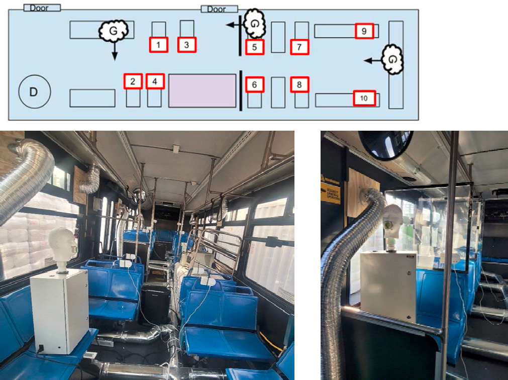
Stationary Testing with Passengers
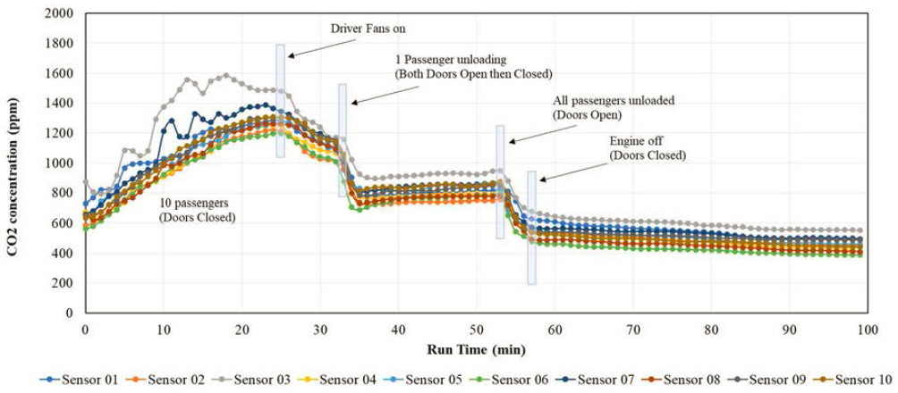
A stationary test using ten passengers was conducted with Bus B. The AC system was powered on to high and set to 60-63 °F inside the cabin. Sensors #1-#10 recorded CO2 concentration levels throughout the testing. The bus doors were open prior to passenger loading during installation of sensors. Once all passengers boarded the bus, the doors were closed. Sitting location was random and selected individually by the passenger (Figure 43). The CO2 concentrations, seen in Figure 44, shows a steady increase from an average of 668 ppm to 1291 ppm during the first 25 minutes. Sensors #3 and sensor #7 recorded higher CO2 levels than other sensors during this period likely due to those nearby passengers continuously speaking more compared to passengers near sensors #5 and #6. At minute 25 the driver fans and blower on the left and front control panel respectively were set to high. This caused a decrease in overall CO2 concentrations throughout the cabin. At minute 33, one passenger was unloaded from the bus where both doors were opened and closed within one minute. The CO2 concentration is observed to decrease over a 3-minute period from an average of 1004 ppm to 790 ppm followed by an increase again to an average value of 832 ppm after 16 minutes. Both doors were opened at minute 53 and passengers exited the bus. This activity caused a rapid decrease in CO2 levels to 561 ppm. Lastly, the bus engine and AC system was turned off and the CO2 concentration depleted to a background level of 464 ppm while the doors remained closed.
Bus cabin air quality is a balance among internal sources of emissions, filtration, and dilution. This parking lot test with passengers in this section demonstrates the importance of bringing outside air into the cabin by fan. As shown previously when a vehicle is in motion the dynamic pressure difference causes outside air to penetrate into the bus cabin. This helps suppress the increase of CO2 exhaled by passengers. In the real world, especially on the busy arterial roads, outside air can contain high concentrations of pollutants (CO2, CO, VOC, particulates, and NOx). In that case, it is required that the ventilation inlet of the bus has a filtration system to remove the outside pollutants before getting into bus cabin because otherwise passengers could be exposed to fresh pollutants coming from outside.