Protecting Transportation Employees and the Traveling Public from Airborne Diseases (2024)
Chapter: 5 CFD Studies of Subway and Tram Cars
Chapter 5
CFD Studies of Subway and Tram Cars
Methods
In this section, CFD simulations are used to investigate the efficacy of incorporating barriers and implementing a parallel ventilation system in reducing the travel distance of airborne particles within two other modes of public transportation—specifically, a subway car and a tram. The study involves a comparative analysis between the baseline scenario and modified models equipped with barriers and/or a parallel flow ventilation system.
Geometric Models
The models employed in this study were sourced from GrabCAD, specifically a subway and a tram, as detailed in Saxena (2019) and ARI (2017), respectively. Careful consideration was given to ensure that these models encompassed key features, including but not limited to HVAC designs, seating arrangements, door configurations, and overall geometry that aligns with those commonly used in the United States.
To maintain a realistic representation, the HVAC systems in both models induce downward airflow and incorporate a return vent, typically situated at the top of each end of the subway or tram section. Seating arrangements were designed to mirror the orientation of contemporary U.S. subway and tram configurations. In the case of the subway, seats are aligned against the walls along the length of the subway, with doors separating each section. For the tram, individual seating is arranged with a minimum of two seats per row, facing perpendicular to the tram’s longest length.
The overall geometry of each model captures essential features of modern transportation. In the subway model, interconnected cart doors are at each end of the cart, with multiple entering and exiting side doors along the length. Similarly, the tram model consists of a two-section cart with multiple side doors for convenient ingress and egress. The geometric dimensions of these models, crucial to the study, are presented in Table 22.
Table 22: Dimensions of subway and tram.
| Model | Length (m) | Width (m) | Height (m) |
|---|---|---|---|
| Subway | 22.5 | 2.98 | 2.73 |
| Tram | 20.8 | 2.65 | 2.89 |
Configurations for Test Subject
The analysis of results is based on four distinct configurations designed to ascertain the impact of incorporating barriers and/or parallel ventilation systems on minimizing the travel distance of particles originating from a cough. All simulations will maintain gravity as a standard parameter. The study is conducted in a static external environment, devoid of thermal effects. It is assumed that only one section of each mode of transportation is under investigation, with the subway featuring a single kart and the tram comprising one section with two adjoining carts, sharing a common ventilation system.
The baseline scenario represents Case 1, conducted without any modifications. Subsequently, Cases 2 through 4 introduce modifications, accompanied by corresponding inlet and outlet adjustments. In the case of parallel vent simulations (Cases 3 and 4), the vent outlet is directed towards the ground, diverging from
the unmodified version where it is positioned at the top. A detailed overview of the four test configurations is presented in Table 23 below.
| Configuration | Flow Direction | Barriers | Parallel Vent |
|---|---|---|---|
| Case 1 (Baseline) | Down | N | N |
| Case 2 (Barriers) | Down | Y | N |
| Case 3 (Parallel Vent) | Down | N | Y |
| Case 4 (Barriers + Parallel Vent) | Down | Y | Y |
Ventilation Modeling
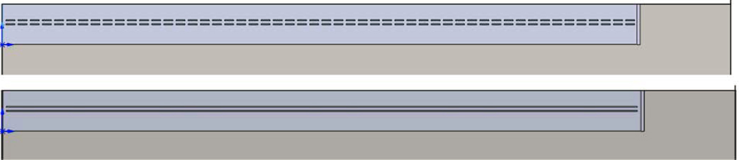
In each scenario, the HVAC system underwent modifications, adopting an approach akin to the one employed in the bus simulation to enhance computational efficiency. The ventilation holes were transformed into elongated slit inlets/outlets, departing from the conventional multi-hole design. Utilizing these extended slits streamlined the simulation process by reducing calculating parameters, thereby achieving comparable outcomes in less time.
The intricate HVAC systems of both the subway and tram encompass features such as air recirculation, air and heating conditioning, and the introduction of fresh exterior air into each carrier section. To simplify the simulation, all inlets and outlets of the ventilation system were amalgamated to yield equivalent flowrates. In addition to consolidated flowrates, the model incorporated the use of long slits instead of multiple smaller slots. Despite this adjustment, the combined flowrates maintain the same volume as the subdivided flowrates, as the total volume entering the model remains constant. Opting for elongated slits over multi-slots not only produces highly comparable results but also significantly expedites computational time (Figure 106).
Barrier Modeling
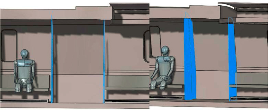
Barriers have been incorporated in tandem with the models to investigate their potential impact on reducing the travel distance of airborne particles. In the case of the subway, barriers were positioned at the end of each seat, aligning with door openings. These subway barriers are visually represented and highlighted in blue in Figure 107. This configuration aims to capitalize on the spatial dynamics within the subway, leveraging the barriers to influence the direction of airflow and enhance particle containment.
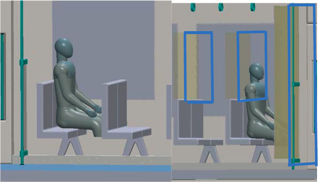
For the tram model, a novel seating geometry allows for the placement of barriers directly on top of the backrest of the seats. The positioning of these barriers is depicted in Figure 108. This innovative approach is designed to optimize the tram’s layout, effectively introducing barriers at a strategic location to influence airflow patterns and enhance particle capture. By integrating barriers into both the subway and tram models, this study seeks to discern the effectiveness of such modifications in curtailing the airborne travel distance of particles.
Parallel Flow Ventilation
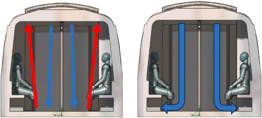
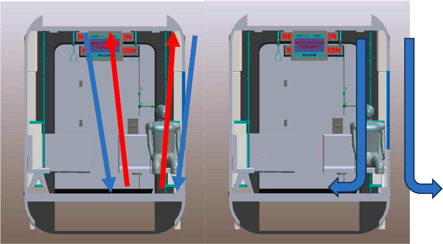
The unaltered ventilation model features an inlet and outlet positioned at the top of the model, requiring the air within the subway and tram to travel upward before exiting. In a bid to reduce the travel distance of the inlet air, a parallel system was introduced. This parallel flow system incorporates air inlets at the top of the model while facilitating exits at the bottom side walls. Figures 109 and 110 illustrate a projection of the air streamlines under normal operation for the subway and tram, respectively.
In these figures, the arrows representing the inlet flow trajectory in the unmodified ventilation system indicate a recirculation of air back toward the top of the model before ultimately exiting. Conversely, the projection of the parallel flow system demonstrates a direct exit at the bottom, eliminating the need for the airflow to traverse back toward the top to locate the outlet vent. This design modification is aimed at streamlining the airflow path and minimizing the overall travel distance within the transportation model.
Flow Rates
The flow rates employed in this study are derived from analogous parametric CFD investigations documented in Tao et al. (2019), Chang et al. (2021), and Suarez et al. (2017). Calculations for the flow rates were determined using the equation below, which leverages the cross-sectional area to ascertain the velocity inlet of the vent. The corresponding values are outlined in Table 24.
Q=VA (Equation 11)
Table 24: Flowrate and Output Cross section Area.
| Model | Flowrate Q (m3/s) | Mean Velocity V (m/s) | Cross-sectional Area A (m2) |
|---|---|---|---|
| Subway | 2.77 | 1.37 | 2.02 |
| Tram | 0.83 | 1.04 | 0.8 |
Computational Model
To ensure accurate simulations and derive meaningful outcomes, the study adopted a k-epsilon (k-є) turbulence model. The k-є model, a two-equation model, effectively considers the convection and diffusion of turbulent energy. This model employs two equations that incorporate the quantifying parameters of kinetic energy (k) and turbulence dissipation rate (є) in the simulation, aiming to emulate a realistic domain in a real-world scenario. The solutions to the k-є model are governed by a set of eight equations. The calculated parameters for each model, pertaining to both the subway and tram, are detailed in Table 25 and Table 26.
(Equation 12)
(Equation 13)
(Equation 14)
(Equation 15)
(Equation 16)
(Equation 17)
(Equation 18)
(Equation 19)
Table 25: K-є parameters of Subway.
| Turbulence Conditions (Subway) | |||||
|---|---|---|---|---|---|
| Terms | Variable | Inside Sub | Inlet Vents | Cough | Units |
| Turbulent Energy [k] | k | 0.345 | 55.998 | 1315.6 | m2/s2 |
| Turbulent Dissipation [ε] | ε | 0.196 | 4988.48 | 4409837.7 | m2/s3 |
| Turbulence Length Scale [l] | L | 0.170 | 0.01386 | 0.00178 | m |
| Turbulence Intensity [I] | I | 4.80 | 4.70 | 4.94 | % |
| Mean Flow Velocity | U | 0.1 | 1.37 | 6 | m/s |
| Characteristic Length | L | 2.43 | 0.20 | 0.0254 | m |
| Turbulence Constant | Cµ | 0.09 | 0.09 | 0.09 | - |
| Kinematic Viscosity of Air | µ | 1.50E-05 | 1.50E-05 | 1.50E-05 | m2/s |
| Density of Air | ρ | 1.2 | 1.2 | 1.2 | kg/m3 |
| Velocity | v | 0.1 | 1.37 | 6 | m/s |
| Hydraulic Diameter | dh | 2.43 | 0.198 | 0.0254 | m |
| Reynolds Number | Re | 15978 | 18016 | 12192 | - |
Table 26: K-є parameters of Tram.
| Turbulence Conditions (Tram) | |||||
|---|---|---|---|---|---|
| Terms | Variable | Inside Tram | Inlet Vents | Cough | Units |
| Turbulent Energy [k] | k | 0.337 | 39 | 1315.6 | m2/s2 |
| Turbulent Dissipation [ε] | ε | 0.180 | 3573.23 | 4409837.7 | m2/s3 |
| Turbulence Length Scale [l] | L | 0.178 | 0.0112 | 0.00178 | m |
| Turbulence Intensity [I] | I | 4.74 | 5.00 | 4.94 | % |
| Mean Flow Velocity | U | 0.1 | 1.04 | 6 | m/s |
| Characteristic Length | L | 2.55 | 0.16 | 0.0254 | m |
| Turbulance Constant | Cµ | 0.09 | 0.09 | 0.09 | - |
| Kinematic Viscosity of Air | µ | 1.50E-05 | 1.50E-05 | 1.50E-05 | m2/s |
| Density of Air | ρ | 1.2 | 1.2 | 1.2 | kg/m3 |
| Velocity | v | 0.1 | 1.04 | 6 | m/s |
| Hydraulic Diameter | dh | 2.55 | 0.16 | 0.0254 | m |
| Reynolds Number | Re | 16767 | 10941 | 12192 | - |
Meshing
The computational domain serves as the physical space where simulation calculations take place, and within this domain, mesh cells play a crucial role by dividing it into smaller sections. The control of the number of cells in a simulation is instrumental in achieving higher resolution in the simulation results. To verify the adequacy of mesh count, a mesh study is conducted, comparing a selected parameter. The attainment of similarity in the parameter across different mesh sizes indicates convergence.
In the study of the subway and tram, a probing line is introduced at shoulder height, running the entire length of the transportation model. This line serves as a measurement point for air velocity in the mesh study. Positioned as close to the center of the model as possible, the line is adjusted to circumvent any obstructions. For the subway, this adjustment is necessary to avoid the posts running down the middle of the model, as illustrated in Figure 111 and Figure 112, which depict the line’s location. The probing line is instrumental in determining the average velocity for the simulation, with each change in mesh cell count. An average change in velocity of less than 5% is deemed acceptable for this study, signifying convergence.
In addition to the middle line velocity, a top vent velocity line is established at the inlet of the vent to validate the inlet velocity. This supplementary line ensures the correctness of the inlet velocity in alignment with the mass flow rate over the specified surface inlet area. Serving as a second verification point, the top vent velocity line enhances confidence that the models align with the measured or calculated values input into the system.


The mesh study will exclusively focus on a baseline model. The locations of the inlet and outlet vents are illustrated in Figure 113 and Figure 114. In the subway model, there are four inlet locations—two positioned on the edges and two running down the middle of the ventilation system. The return or exit location is situated at the top of the system and comprises six locations, with two at the front, two in the middle, and two at the rear. The geometry of the vents was designed based on Figure 2 in Y. Tao et al. (2019, 329-336). The vent geometry incorporates side inlets as well as direct inlets facing downward towards the cabin of the subway.

The tram model features four vent inlets, with two on each cart positioned on both sides and running the entire length of the kart. The outlet vent for the tram is specifically located in the initial section of the connecting kart, towards the connection point of the two karts. Figure 114 illustrates the model’s vent inlet and outlet locations, highlighted in blue and circled in red. Our approach with this work followed that of Suarez et al. (2017).

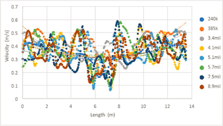
The subway’s mesh study encompasses a total of eight simulations, with the average velocity serving as the key parameter for measurement. In Table 27, the mesh sizes utilized for each simulation, along with specific mesh settings, are detailed. Figure 115 presents an overlay of the results from each simulation. The graph reveals varying velocities for each simulation based on mesh size. To discern the differences between each line, a line of best fit employing a polynomial function is applied. The average area under the curve is employed for a comprehensive comparison of the average differences between each line. The plot showcases the integration of the area below the graph, ultimately yielding the average velocity. The equations utilized are outlined as follows:
(Equation 20)
(Equation 21)
(Equation 22)
(Equation 23)
Table 27: Mesh settings used in each Subway simulation.
| Mesh Level | Mesh Cells | Fluid Cells Contacting Solids | Nx | Ny | Nz | Refining Cells Level (Fluid/Fluid Solid Boundary) | Iterations |
|---|---|---|---|---|---|---|---|
| 1 | 235,230 | 91,225 | 8 | 6 | 54 | 2/2 | 124 |
| 2 | 385,541 | 173,649 | 8 | 6 | 54 | 2/2 | 146 |
| 4 | 3,363,682 | 1,898,918 | 24 | 18 | 180 | 0/0 | 300 |
| 4 | 4,093,223 | 1,943,219 | 26 | 26 | 200 | 1/1 | 320 |
| 5 | 5,175,292 | 1,950,515 | 34 | 34 | 275 | 1/1 | 346 |
| 5 | 5,696,286 | 2,241,092 | 34 | 34 | 275 | 1/2 | 358 |
| 5 | 7,493,504 | 2,627,229 | 40 | 40 | 300 | 1/2 | 396 |
| 6 | 8,887,663 | 2,912,573 | 34 | 34 | 290 | 1/1 | 415 |

Results
Having established the average velocity, a comparative analysis is conducted by examining the velocity of each mesh size in relation to the next larger mesh size. The percentage difference between the two is calculated for comparison, and the results are presented in Table 28. Mesh sizes deemed ideal for the subway simulation are highlighted in green on the right of the table (see also Figure 116). The highlighted percentage values indicate instances where the change between simulations is less than 5%, signifying that these mesh sizes are considered optimal for this study. Based on these results, 5.1 million cells was used for the subway simulations.
| Cell Count | Average (m/s) | Velocity Difference (m/s) | Percent Difference (%) |
|---|---|---|---|
| 240k | 0.34549 | x | x |
| 385k | 0.395 | 0.050 | 14.390 |
| 3.4mil | 0.399 | 0.004 | 0.890 |
| 4.1mil | 0.345 | -0.054 | 13.539 |
| 5.1mil | 0.356 | 0.011 | 3.148 |
| 5.7mil | 0.359 | 0.003 | 0.972 |
| 7.5mil | 0.346 | -0.014 | 3.773 |
| 8.9mil | 0.354 | 0.008 | 2.321 |
The top ventilation was meticulously considered during the meshing process, ensuring that the air inlet speed aligns with the prescribed calculated value. To verify this alignment, a plot was positioned at the ventilation inlets to measure the mesh’s capability to accurately gauge and inject the flow rate at the intended velocity. Figure 117 below serves as validation, indicating that the mesh size is indeed sufficient for the
subway CFD simulation. The percentage difference observed is less than 1% from the reference value in Table 25, which specifies an inlet speed of 1.37 m/s.

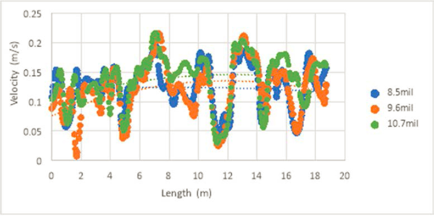
The mesh study for the tram adheres to a structure similar to the subway mesh study. It involves eight distinct mesh sizes, with convergence observed at approximately 8.5 million cells. The tram model, characterized by a more intricate level of detail compared to the subway, tends to necessitate a higher mesh density. Table 29 provides an overview of the various mesh sizes and their corresponding variable settings. Figure 118 and Figure 119 visually represent the overlay of velocity graphs for comprehensive understanding.
Table 29: Mesh settings used for each tram simulation study.
| Mesh Level | Mesh Cells | Fluid Cells Contacting Solids | Nx | Ny | Nz | Refining Cells Level (Fluid/Fluid Solid Boundary) | Iterations |
|---|---|---|---|---|---|---|---|
| 2 | 7.0E+05 | 3.6E+05 | 10 | 10 | 78 | 1/1 | 178 |
| 2 | 3.2E+06 | 1.7E+06 | 10 | 10 | 78 | 1/1 | 294 |
| 3 | 4.7E+06 | 2.4E+06 | 16 | 16 | 122 | 1/1 | 334 |
| 4 | 6.0E+06 | 3.0E+06 | 22 | 22 | 170 | 1/1 | 364 |
| 5 | 7.5E+06 | 2.8E+06 | 34 | 34 | 260 | 1/2 | 392 |
| 5 | 8.5E+06 | 3.2E+06 | 36 | 36 | 265 | 1/2 | 409 |
| 6 | 9.6E+06 | 3.0E+06 | 38 | 38 | 280 | 1/2 | 426 |
| 6 | 1.1E+07 | 3.5E+06 | 40 | 40 | 290 | 1/2 | 442 |

As outlined in Table 30, the optimal mesh count for the tram simulation appears to be 8.5 million cells. Notably, at 9.6 and 10.7 million cells, the velocity difference also remains below 5 percent, aligning with the acceptable range within the context of the simulations. The percentage differences are visually highlighted in green on the right side of the table for quick identification and reference.
Table 30: Average velocity and difference of the previous simulation on the tram simulations.
| Cell Count | Average (m/s) | Velocity Difference (m/s) | Percent Difference (%) |
|---|---|---|---|
| 701k | 0.094 | x | x |
| 3.1mil | 0.113 | 0.019 | 20.130 |
| 4.6mil | 0.120 | 0.007 | 6.136 |
| 6mil | 0.134 | 0.014 | 12.093 |
| 7.5mil | 0.142 | 0.008 | 5.774 |
| 8.5mil | 0.122 | -0.020 | 13.781 |
| 9.6mil | 0.120 | -0.002 | 1.539 |
| 10.7mil | 0.125 | 0.005 | 3.769 |
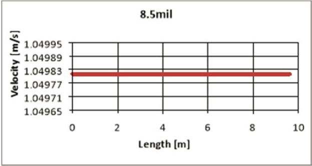
Following a pattern akin to the subway study, the inlet velocity of the top vent in the tram simulation exhibits an optimal consistency with less than a 5% difference in velocity. Specifically, the tram’s inlet velocity percentage difference is impressively below 1% of the value provided in Table 30. These results strongly suggest that the mass flowrate is accurately and effectively represented in the study.
Particle Injection
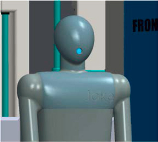
In this study, mannequins are employed to simulate the release of 100 particles with a size of 1 micron each, originating from the mouth orifice. To replicate a coughing scenario, an initial inlet velocity of 6 meters per second was applied at the mouth orifice. Subsequently, as these particles are expelled into the environment, their airborne trajectories were tracked, and the distance traveled along the lengthwise axis of the transportation was quantified and set into predetermined zones.
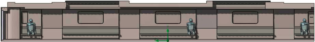
Figure 121 provides a visual representation of the starting locations from the mannequin’s orifice. For the subway study, three mannequins were strategically placed in the front, middle, and rear of the subway, each positioned in a seated posture. In the tram study, four mannequins were distributed at the front, one-third from the front, two-thirds from the front, and the rear position of the tram. The specific locations of these mannequins are depicted in Figure 122.

To conduct a comprehensive analysis of the results, both the subway and tram need to be segmented into distinct sections of interest. These sections are delineated based on the zone of occupancy, with each row of seating signifying a specific section. In instances where there is no designated seating arrangement, the sections were demarcated to correspond to areas representing openings or connections between carts, if present in the model. The graphical representation of these sections is provided in Figure 123.

Each particle injected for the study undergoes a fate of either absorption into the environment or remaining in an open state. Absorption signifies that the particle has collided with a geometric feature within the model, marking the conclusion of its travel distance. On the other hand, particles in the open state are still airborne at the conclusion of the simulation or have exited the interior cabin of the model through the outlet vent. Given the high occurrence rate of particles in the open state leaving the system through the outlet ventilation, the fate of opening particles were factored into the results. Consequently, only absorbed particles and their corresponding zones of landing were considered in the analysis.
Computing Particle Distance Travel
SOLIDWORKS incorporates a built-in particle study function that provides the capability to monitor various parameters such as the travel length, trajectory, and starting/ending positions of particles. Utilizing this function, the data of each particle’s ending location can be extracted and employed to illustrate the disbursement of particles within the model.
The subway study results suggest that the incorporation of barriers and parallel ventilation has minimal impact. In all scenarios, absorbed particles tend to remain within the zones into which they were initially injected, irrespective of the baseline or modified conditions. The total absorbed particles in the baseline, barriers, parallel flow, and parallel flow/barriers scenarios are 143, 245, 167, and 143 particles, respectively (Figure 124). Notably, the barrier simulation exhibits a higher overall absorption rate within the model. The addition of barriers created a case of leaving particles exposed for passengers to contact.
The desired outcome would be for most of the particles to exit the system, remaining in an open state rather than being absorbed within the subway. However, several factors contribute to the limited effect of barriers and parallel flow ventilation on the particle’s travel path and absorption rate. One significant factor is the presence of multiple outlet ventilation ports throughout the subway, resulting in particles having a shorter total travel distance to reach the outlet. Another contributing factor is the placement of the mannequins, positioned in close proximity to the outlet vent. This placement leads to the exiting air pulling the 1-micron particles into the airstream, creating a condition where particles leave the internal cabin, contributing to an open state in the simulation results. Lastly, the geometry of the subway proved hard to add effective barrier boundaries without impeding traffic flow within the subway.

The tram study demonstrates that the integration of a parallel ventilation system and barriers effectively reduces the travel distance of airborne particles. Zones 7 and a portion of zone 8 correspond to the baseline exit vent location. As illustrated in Figure 125, the baseline study reveals that 136 particles land in zones 7 and 8, suggesting that airborne particles align with air streamlines and exit path trajectories, falling short of the outlet vent in these zones.

Notably, zones 11, 12, and 13 exhibit a slight increase in particle absorption with the introduction of barriers and the parallel ventilation system. This rise is presumed to be influenced by the seating orientation of the rear injection, which faces the width of the tram rather than the length. Adjusting the rear seat orientation to face forward is expected to correlate with a lower absorption rate in zones 11 to 13.
In summary, the subway simulation reveals minimal changes, contrasting with the tram model that demonstrates highly effective alterations. The results highlight a significant reduction in particles landing throughout the tram, underscoring the effectiveness of parallel ventilation and barriers. This reduction implies a decreased number of airborne particles traveling through other zones, emphasizing the efficacy of incorporating barriers and parallel ventilation systems in trams.


