Design of Piles for Downdrag (2024)
Chapter: 2 Execute Methodology
SECTION 2
Execute Methodology
2.1 Introduction
Two methods are prescribed for identifying the location of the neutral plane and determining the amount of downdrag and resulting drag load. These two methods include Method A, an analysis method based on the use of fully mobilized load transfer discussed in detail in Section 2.5.1 of this report, and Method B, an analysis method based on the use of partially mobilized load transfer discussed in detail in Section 2.5.2. For both Methods A and B, several techniques are described for determining the appropriate soil parameters for use in design. These prescribed techniques are drawn from Geotechnical Engineering Circular No. 5: Geotechnical Site Characterization (Loehr et al. 2016). For Method A, the static axial resistance estimation methods described in the AASHTO (2020) specification are provided for completeness. These resistance estimation methods were used to determine the load and resistance curves that are required for identifying the location of the neutral plane and determining the amount of drag load developed.
For Method B, a database of 68 static load tests on instrumented piles, which have been obtained from documented literature, has been developed to support the proposed drag load evaluation methodology. The load transfer from these instrumented piles to the surrounding soil, including side and toe-bearing resistance, has been developed from the reported pile head load-displacement and load transfer data and is documented in the database. The pile database includes the following types of piles: steel pipe, steel H, concrete-filled steel pipe, concrete square, concrete cylinder, and concrete H. The residual load for each pile was estimated to correct for the influence of residual load on the developed side and toe-bearing resistance of each pile. In several cases where measured residual load data exists, the estimated residual load has been compared to the residual load reported by those who conducted the static loading test.
Data from several of the piles in the database were used to predict the location of the neutral plane and estimate the amount of drag load expected in the pile. Moreover, in an effort to demonstrate the developed Method B, a static loading test of a steel pipe pile has been simulated using commercially available load transfer simulation software. The load transfer measured at each strain gauge location along the pile and the specified pile head loads have been used as input in the analysis to simulate the load transfer of the pile. The results are compared to a similar analysis where the residual load-corrected load transfer data were used as input to the software to demonstrate the effect of the estimated residual load. Following the simulation of the residual load, the drag load on the pile was simulated considering the settlement of the soil profile as a function of depth. Distributions of the load transfer along the pile and the location of the neutral plane in the pile are also described.
2.2 Selection of Soil Correlations
To facilitate comparisons between field t-z curves and existing t-z curve models and to correct for residual pile loads, correlations from reported field tests and laboratory data to soil design parameters were selected and are presented in the following sections. For the pile tests included in the pile load test database, either standard penetration tests (SPTs) or cone penetration tests (CPTs) were typically reported. Several tests also reported laboratory data, including sieve analysis, Atterberg limits, and unconfined compression tests. For test cases including multiple types of in situ tests (CPT and SPT), CPTs were preferred for determining soil design parameters. Similarly, when laboratory and field tests were available, the laboratory tests were preferred for establishing design parameters.
AASHTO (2020) generally does not prescribe specific correlations for the selection of soil design parameters. However, AASHTO (2020) does require the use of Bowles (1977) (Tables 2.2.1 and 2.2.2) for determining the drained friction angle of granular soils from SPTs and provides a correlation for Poisson’s ratio and maximum shear modulus based on soil type and consistency. Furthermore, AASHTO (2020) frequently directs practitioners to the earlier Geotechnical Engineering Circular No. 5: Evaluation of Soil and Rock Properties (Sabatini et al. 2002) for guidance regarding subsurface investigations, in situ testing, and selection of design parameters. An updated version of the Geotechnical Engineering Circular No. 5 was released in 2016 (Loehr
Table 2.2.1. Correlations from SPT blow counts to design parameters for granular soils.
| Parameter | Reference | Correlation | Notes |
|---|---|---|---|
| Friction angle, ϕ' (deg) | Bowles (1977) | Presented in Table 2.2.3 | Granular soils |
| Hatanaka and Uchida (1996) | Fine to medium sands | ||
| Kulhawy and Chen (2007) | ϕ' = 27.5 + 9.2 log [(N1)60] | Sands and gravels | |
| Unit Weight, γ (pcf) | Vanikar (1986) | Presented in Table 2.2.3 | |
| Shear Modulus, Gmax (psf) | Seed et al. (1986) | ||
| Poisson’s Ratio, v | NAVFAC (1982) | Presented in Table 2.2.5 | |
NOTE: pcf = pounds per cubic foot; psf = pounds per square foot.
Table 2.2.2. Correlations from SPT blow counts to design parameters for plastic soils.
| Parameter | Reference | Correlation | Note |
|---|---|---|---|
| Shear Strength, su (psf) | Loehr et al. (2017) | Find S and m from Table 2.2.6 | |
| Preconsolidation Pressure, (psf) | Mayne and Kemper (1988) | (kPa) | |
| Unit Weight, γ (pcf) | Vanikar (1986) | Presented in Table 2.2.4 | |
| Elastic Modulus, Es | NAVFAC (1982) | Presented in Table 2.2.5 | |
NOTE: kPa = kilopascal.
Table 2.2.3. Correlation of SPT N1,60 values to drained friction angle and unit weight [modified from AASHTO (2020) and Vanikar (1986), respectively]. Originally adapted from Bowles (1977).
| Soil Description | Corrected Blow Count, N1,60 (blows/ft) | Effective Friction Angle ϕ' (deg) | Unit Weight, γ pcf |
|---|---|---|---|
| Very Loose | <4 | 25–30 | 70–100 |
| Loose | 4 | 27–32 | 90–115 |
| Medium | 10 | 30–35 | 110–130 |
| Dense | 30 | 35–40 | 110–140 |
| Very Dense | 50 | 38–43 | 130–150 |
et al. 2016). For the selection of soil design parameters, the research team utilized the guidance provided in AASHTO (2020) whenever possible. However, rather than referencing Sabatini et al. (2002) for guidance, the 2016 version of Geotechnical Engineering Circular No. 5 (hereafter referred to GEC No. 5) was used (Loehr et al. 2016).
2.2.1 In Situ Test Correlations: SPT
For SPT data, correlations were selected for granular and plastic soils (Tables 2.2.1 and 2.2.2, respectively). The correlation from corrected SPT blow count to effective friction angle presented in Table 2.2.3 is the correlation currently prescribed by AASHTO (2020); however, the Bowles (1977) correlation tends to provide conservative values for effective friction angle. Therefore, two alternative correlations have been selected; specifically, Hatanaka and Uchida (1996) and Kulhawy and Chen (2007) were selected for fine to medium sands and for other sands and gravels, respectively. Hatanaka and Uchida (1996) was recommended by GEC No. 5 (Loehr et al. 2017) and used triaxial tests of high quality, fine to medium sand samples obtained via soil freezing to develop their correlation. Due to the limits of the materials tested by Hatanaka and Uchida (1996), a second correlation was selected for use with coarse sands and gravels; specifically, Kulhawy and Chen (2007) was selected because their correlation was developed utilizing a broad range of sands and gravels (57 different samples). A comparison of the three friction angle correlations is presented in Figure 2.2.1.
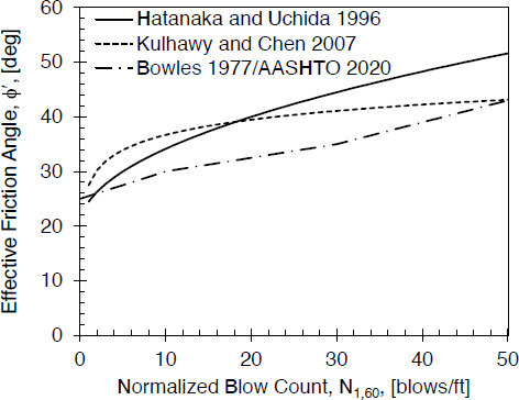
Table 2.2.4. Empirical relationship between SPT values to unit weight for plastic soils [modified from Vanikar (1986)].
| Consistency | Very Soft | Soft | Medium | Stiff | Very Stiff | Hard |
|---|---|---|---|---|---|---|
| Blow Count, N60 | 0 | 2 | 4 | 8 | 16 | 32 |
| Unit Weight, γ pcf | 100–120 | 110–130 | 120–140 | 140 | ||
The SPT blow count to unit weight correlation selected for plastic and granular soils was Vanikar (1986), an extension of the Bowles (1977) correlation that is included in AASHTO (2020) for friction angle (Table 2.2.4). Similarly, the existing correlation included in AASHTO (2020) for Poisson’s ratio and the elastic modulus for plastic soils was selected (Table 2.2.5). For determining shear modulus, a correlation presented in GEC No. 5 (Loehr et al. 2017) was selected for use, specifically, the Seed et al. (1986) method.
Determining soil shear strength from SPT blow counts is an unadvisable practice; however, when no laboratory or other field data are available, a means to determine the shear strength of plastic soils is needed. The GEC No. 5 (Loehr et al. 2017) recommended utilizing SHANSEP (Stress History and Normalized Engineering Properties) to determine shear strength. Some criteria for SHANSEP parameters are presented in Table 2.2.6 (Ladd and DeGroot 2003). Generally, for low-plasticity clays the parameters S and m can be taken as 0.2 and 1.0, respectively. For high plasticity clays, S and m can be taken as 0.22 and 0.8, respectively. Finally, to determine shear strength from SPT blow counts, Mayne and Kemper (1988) was selected to determine the overconsolidation ratio (OCR). The correlation to preconsolidation pressure was selected rather than correlating directly to OCR due to the improved correlation.
Table 2.2.5. Typical values for Young’s modulus and Poisson’s ratio for different soil types [from AASHTO (2020)].
| Soil Type | Typical Range of Young’s Modulus, Es (ksi) | Poisson’s Ratio, v |
|---|---|---|
| Soft Sensitive Clay | 0.347–2.08 | |
| Medium-Stiff to Stiff Clay | 2.08–6.94 | 0.40–0.50 (undrained) |
| Very Stiff Clay | 6.94–13.89 | |
| Loess | 2.08–8.33 | 0.10–0.30 |
| Silt | 0.278–2.78 | 0.30–0.35 |
| Loose Fine Sand | 1.11–1.67 | |
| Medium-Dense Fine Sand | 1.67–2.78 | 0.25 |
| Dense Fine Sand | 2.78–4.17 | |
| Loose Sand | 1.39–4.17 | 0.20–0.36 |
| Medium-Dense Sand | 4.17–6.94 | — |
| Dense Sand | 6.94–11.11 | 0.30–0.40 |
| Loose Gravel | 4.17–11.11 | 0.20–0.35 |
| Medium Dense Gravel | 11.11–13.89 | — |
| Dense Gravel | 13.89–27.78 | 0.30–0.40 |
NOTE: — = not reported.
Table 2.2.6. SHANSEP parameters for different plastic soils [from Ladd and DeGroot (2003)].
| Soil Description | S | m† | Remarks |
|---|---|---|---|
|
S = 0.20 (σ ≈ 0.015)‡ |
m = 1.00 | Champlain clays of Canada |
|
No shells or sand lenses/layers | ||
|
S = 0.16 | m = 0.75 | Assumes DSS mode of failure |
|
S = 0.25 (σ = 0.05) |
Excludes peat |
†m = 0.88 (1 − Cs/Cc) based on CKoUDSS tests for 13 solis with max OCR of 5 to 10
‡σ denotes standard deviation
NOTE: DDS = direct simple shear.
2.2.2 In Situ Test Correlations: CPT
Correlations to granular and plastic soil properties using the CPT were selected (Table 2.2.7 and 2.2.8, respectively). When no correlation for a particular design parameter was available in AASHTO (2020) or Loehr et al. (2017), the 6th edition of Guide to Cone Penetration Testing for Geotechnical Engineering (Robertson and Cabal 2015) was utilized. Similar to the correlation provided in GEC No. 5 (Loehr et al. 2017) for SPT to friction angle, the CPT to friction angle correlation is based on limited data. Specifically, the procedure proposed by Kulhawy and Mayne (1990) is appropriate for clean sands only. Therefore, a second correlation (Robertson and Cabal 2015) for other sands was selected for sands with gravels and/or fines.
The correlations for Poisson’s ratio and elastic modulus are the same correlations presented for correlating to SPT data. The correlation for shear modulus of granular soils was selected from GEC No. 5. The unit weight correlation for both granular and plastic soils came from Robertson and Cabal (2015). The same SHANSEP methodology used in the SPT correlation was selected for determining the shear strength of soil, rather than using the Nkt method, for which the
Table 2.2.7. Correlations from CPT blow counts to design parameters for granular soils.
| Parameter | Reference | Correlation | Note |
|---|---|---|---|
| Friction Angle, ϕ' (deg) | Kulhawy and Mayne (1990) | ϕ' = 17.6 + 11 log(Qtn) | Clean sands |
| Robertson and Cabal (2015) | ϕ' = ϕ'cv + 15.84[log Qtn,cs] − 26.88 | Non-clean sands | |
| Shear Modulus, G (Pa) | Rix and Stokoe (1991) | Use G = ρVs2, Vs in m/sec and qt and σ'v0 in MPa | |
| Poisson’s Ratio, v | NAVFAC (1982) | Table 2.2.5 | — |
| Unit Weight, γ pcf | Robertson (2010) | qt and pa must be in the same units |
Table 2.2.8. Correlations from CPT blow counts to design parameters for plastic soils.
| Parameter | Reference | Correlation | Note |
|---|---|---|---|
| Shear Strength, su | Loehr et al. (2017) | Find S and m from Table 2.2.6 | |
| Preconsolidation Pressure, | Mayne (2017) | — | |
| Elastic Modulus, Es | NAVFAC (1982) | Table 2.2.5 | — |
| Unit Weight, γ | Robertson (2010) | — |
variability in possible Nkt is larger than 100%. The selected preconsolidation pressure correlation is that proposed by Mayne (2017). All of the equations used are provided in Tables 2.2.7 and 2.2.8.
2.3 Comparison of Existing Published t-z Relationships
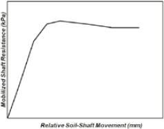
It is well-known that local elastic compression along the shaft of a deep foundation triggers relative soil-pile movement (defined herein as z), which in turn generates interface shearing resistance or side resistance, t, along the pile (Coyle and Reese 1966). Downward elastic compression produces positive relative soil-pile movement and therefore positive side resistance, whereas downward movement of soil relative to pile produces negative soil-pile movement and negative side resistance. The relationship between relative soil-pile movement and side resistance is termed the “t-z curve,” which, if quantified, can be used to prescribe the load transfer along a pile under loading from either the pile head or soil settlement.
Since the possibility of conducting an instrumented static loading test on each project varies, it is common industry practice to utilize published t-z relationships to estimate t-z behavior when site-specific, instrumented static loading tests cannot be conducted. Using the pile load test database collected for this project, it is possible to assess the accuracy of predicted t-z responses utilizing published t-z relationships with observed field responses during static loading tests. Bohn et al. (2017) conducted a similar investigation to assess the accuracy of published t-z relationships. Specifically, the Bohn et al. (2017) investigation assessed “simple” mathematical t-z relationships and proposed two new relationships (a cubic root t-z relationship and a hyperbolic t-z relationship). The Bohn et al. (2017) methodology relied on subjective assessments of the accuracy of t-z relationships rather than utilizing objective statistical analysis.
Six available t-z relationships were selected for investigation based on the work of previous researchers, the use of commonly utilized commercial software, and the prevalence and use in the literature. Specifically, the two relationships (a cubic root t-z relationship and a hyperbolic t-z relationship) proposed by Bohn et al. (2017) were selected for investigation. The three t-z relationships included in common commercial software programs for driven piles (e.g., TZPILE by Ensoft, Inc. and RSPile by Rocscience) were selected and include Coyle and Reese (1966), American Petroleum Institute (API 2002), and Mosher (1984). Finally, the t-z curve proposed by Vijayvergiya (1977) was selected due to the prevalence of the method in literature. A summary of the published t-z curves selected for investigation is included in Table 2.3.1.
In the initial evaluation of t-z relationships, the published t-z relationships were compared against the field-observed t-z responses in the pile database utilizing the maximum observed pile stress for each t-z response. An example of this comparison is presented in Figure 2.3.1,
Table 2.3.1. Summary of selected t-z relationships.
| Reference | Mathematical Expression | Curve Shape | Ground Type | Pile Type |
|---|---|---|---|---|
| API (2002) |  |
 |
Clay and non-carbonate sand | All |
| Coyle and Reese (1966) |  |
 |
Clay | Steel pile |
| Mosher (1984) | 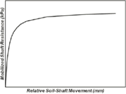 |
Sand | Concrete and steel | |
| Bohn et al. (2017): Cubic Root | 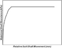 |
All | All | |
| Bohn et al. (2017): Hyperbolic | 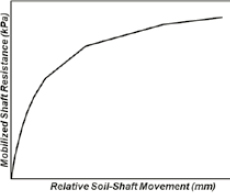 |
All | All | |
| Vijayvergiya (1977) | 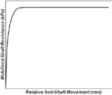 |
Sand and clay | Driven piles |
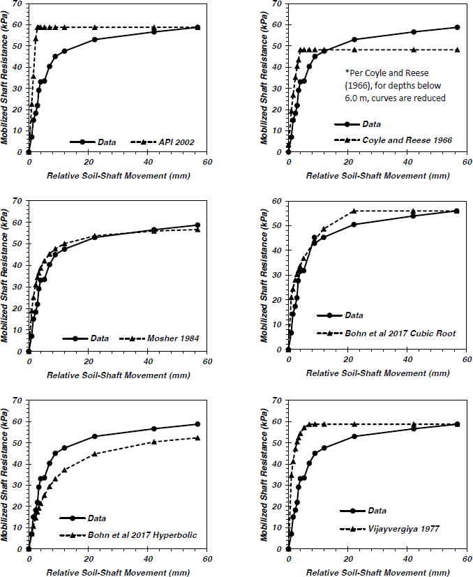
utilizing gauge one of Pile 1 (Bradshaw et al. 2012) in the compiled pile database (see NCHRP Web-Only Document 398, Appendix A). A secondary evaluation utilizing AASHTO recommended static resistance methods (e.g., Meyerhof 1976; Schmertmann 1975; Nordlund 1979; Tomlinson 1980); additionally, the Beta method (Fellenius 1991) and a SHANSEP-based resistance method (Stuedlein et al. 2020) was evaluated. The purpose of the two evaluations was to assess (1) the accuracy of the published t-z curves without the added uncertainty of static design resistance and (2) to evaluate the accuracy of the published t-z responses when combined with static load resistance methods.
Three statistical criteria are used to evaluate the accuracy of the published t-z relationships: (1) the Mean Bias (Equation 2.3.1), (2) the Coefficient of Variation (COV) of Bias (Equation 2.3.2), and (3) the Normalized Root Mean Squared Error (NRMSE) (Equation 2.3.3). These statistical measures are used to assess the goodness-of-fit of the computed t-z curves to the field-observed t-z responses. The accuracy of the selected t-z curves will then be assessed by considering the average of the statistical measures across several bins, specifically, t-z grade (A or B), pile type (steel or concrete), and soil type (plastic or granular) as described below:
| Equation 2.3.1 | |
| Equation 2.3.2 | |
| Equation 2.3.3 |
where yi,o is the observed value at instance i, yi,f is the forecasted value at instance i, n is the total number of instances (number of measured points), SD is the standard deviation, and yo,max is the maximum observed value of y.
The relative quality of each t-z curve (e.g., Grade 1 versus 2) is assessed through inspection of the field observations; specifically, if the tributary area for a given strain gauge is located in a single homogenous soil layer, then the t-z curve is assigned Grade 1 (i.e., there is high confidence that the t-z curve reflects the local soil conditions surrounding the pile). However, a strain gauge influenced by multiple soil layers is assigned Grade 2. The t-z grading criteria are depicted in Figure 2.3.2.
An example of the output table created for the Vijayvergia (1977)-selected t-z relationships is presented in Table 2.3.2. The results for the t-z analysis are included in Appendix B. The accuracy for each t-z relationship can be assessed for each bin and globally. Based on the performance of the t-z relationships, recommendations are made regarding which t-z relationship should be utilized in the absence of an instrumented static load test. A similar analysis will also be conducted for published q-z relationships, which prescribe the unit toe-bearing resistance with toe displacement.
2.4 Collected Database
The driven, static, instrumented pile load test database developed from a review of the literature is presented in Tables 2.4.1 and 2.4.2. Each record includes the measured load-displacement curve of the pile at the pile head as well as the distribution of force (i.e., load transfer) along the pile length for available loading increments. Sixty-eight piles are included in the database: 38 piles are of steel fabrication, whereas 30 piles are constructed of concrete.
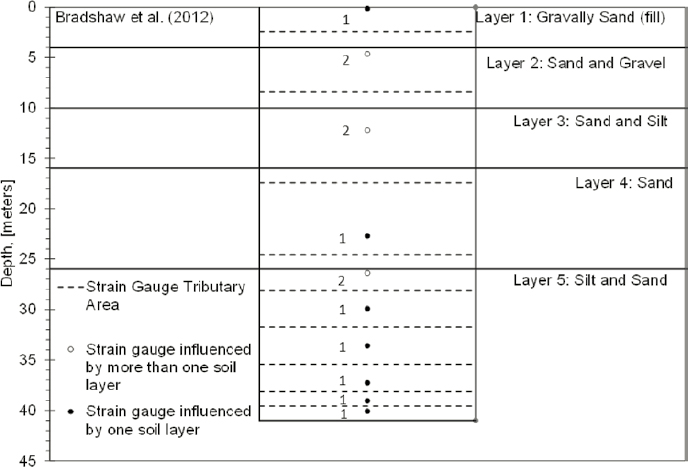
Table 2.3.2. Example summary table for Vijayvergiya (1977).
| Grade | Material | Cohesion | Mean Bias | COV Bias | RMSE |
|---|---|---|---|---|---|
| 1 | |||||
| Steel | Cohesive | 0.8 | 34.3 | 50.50 | |
| Cohesionless | 0.8 | 28.2 | 16.50 | ||
| Concrete | Cohesive | 0.7 | 42.2 | 55.60 | |
| Cohesionless | 0.7 | 37.3 | 17.20 | ||
| 2 | |||||
| Steel | Cohesive | 0.9 | 38.5 | 14.20 | |
| Cohesionless | 0.8 | 33.5 | 26.20 | ||
| Concrete | Cohesive | 0.7 | 35.1 | 9.80 | |
| Cohesionless | 0.7 | 34.9 | 26.90 | ||
Table 2.4.1. Database of the various instrumented pile used to develop load transfer curves.
| General Information | Pile Characteristics | |||||
|---|---|---|---|---|---|---|
| Pile No. | Authors | Location | Type | Total Pile Length (m) | Embedded Pile Length (m) | Width or Diameter (mm) |
| P1 | Bradshaw et al. (2012) | Rhode Island, USA | Open-ended steel pipe piles | 41.60 | 41.00 | 1,830 |
| P2 | Narsavage (2019) | Great Miami River in Dayton, Ohio, USA | Concrete-filled steel pile | 14.00a | 14.00 | 406 |
| P3 | Narsavage (2019) | Great Miami River in Dayton, Ohio, USA | Concrete-filled steel pile | 16.00a | 16.00 | 406 |
| P4 | Petek et al. (2012) | Coquitlam, British Columbia, Canada | Open-ended steel pipe pile | 75.00 | 69.50 | 1830 |
| P5 | Paik et al. (2003) | Lagrange County, Indiana, USA | Closed-ended steel pipe pile | 8.24 | 6.87 | 356 |
| P6 | Seo et al. (2009) | Jasper County, Indiana, USA | Steel H-pile | 18.50 | 17.40 | 310 |
| P7 | Bica et al. (2014) | Jasper County, Indiana, USA | Closed-ended steel pipe pile | 18.50 | 17.40 | 356 |
| P8 | Ng et al. (2013) | Clarke County, Iowa, USA | Steel H-pile | 18.30 | 17.30 | 250 |
| P9 | Ng et al. (2013) | Poweshiek County, Iowa, USA | Steel H-pile | 18.3.0 | 17.40 | 250 |
| P10 | Tee et al. (2019) | Seberang Prai, Penang, Malaysia | Precast reinforced concrete square pile | 42.00 | 41.10 | 400 |
| P11 | Tee et al. (2019) | Seberang Prai, Penang, Malaysia | Precast reinforced concrete square pile | 35.00 | 34.00 | 400 |
| P12 | Altaee et al. (1992) | Baghdad University complex, Iraq | Precast concrete square pile | 12.00 | 11.00 | 285 |
| P13 | Chen et al. (2014) | Vernon Parish, Louisiana, USA | Prestressed square precast concrete pile | 16.80 | 15.20 | 610 |
| P14 | Sun et al. (2020) | Nanjing, China | Pretensioned spun concrete pipe pile | 25.00 | 25.00 | 500 |
| P15 | Suleiman et al. (2010) | Oskaloosa, Iowa, USA | Ultrahigh-performance concrete H-pile | 10.70 | 9.90 | 254 |
| P16 | Haque et al. (2017) | Louisiana, USA | Precast reinforced concrete square piles | 39.60 | 36.60 | 410 |
| P17 | Haque et al. (2017) | Louisiana, USA | Precast, prestressed concrete square pile | 57.90 | 54.90 | 760 |
| P18 | Haque et al. (2017) | Louisiana, USA | Precast reinforced concrete square piles | 48.80 | 45.70 | 610 |
| P19 | Haque et al. (2017) | Louisiana, USA | Precast reinforced concrete square piles | 64.00 | 61.00 | 610 |
| P20 | Haque et al. (2017) | Louisiana, USA | Precast reinforced concrete square piles | 44.20 | 42.40 | 610 |
| P21 | Haque et al. (2017) | Louisiana, USA | Precast reinforced concrete square piles | 51.80 | 49.70 | 610 |
| P22 | Haque et al. (2018) | Louisiana, USA | Precast reinforced concrete square piles | 14.13 | 13.60 | 762 |
| P23 | Haque (2015) | Bayou Lacassine, Louisiana, USA | Precast reinforced concrete square piles | 22.90 | 20.40 | 762 |
| P24 | Haque (2015) | Bayou Lacassine, Louisiana, USA | Precast reinforced concrete square piles | 22.90 | 20.40 | 762 |
| P25 | Yoon et al. (2011) | Caminada Bay, Louisiana, USA | Precast reinforced concrete square piles | 21.00 | 18.56 | 914 |
| P26 | Yoon et al. (2011) | Caminada Bay, Louisiana, USA | Precast reinforced concrete square piles | 22.00 | 19.80 | 914 |
| P27 | Xing et al. (2012) | Jiangsu Province (Site A), China | Prestressed concrete cylinder piles | 40.00 | 40.00 | 600 |
| P28 | Ali and Kai (2013) | Johor, Malaysia | Precast driven concrete cylinder pile | 47.25 | 47.25 | 450 |
| P29 | Leung et al. (1991) | Singapore | Precast square concrete pile | 26.00 | 24.00 | 280 |
| P30 | Leung et al. (1991) | Singapore | Precast square concrete pile | 30.00 | 28.00 | 260 |
| P31 | Briaud et al. (1989) | San Francisco, California, USA | Closed-end steel pipe pile | 10.06 | 9.15 | 273 |
| P32 | Goble et al. (1972) | West Lafayette, Indiana, USA | Steel H-pile | 15.24 | 14.33 | 260 |
| P33 | Tavenas (1971) | St. Charles River, Quebec, Canada | Steel H-pile | 21.00 | 18.20 | 310 |
| P34 | Tavenas (1971) | St. Charles River, Quebec, Canada | Precast concrete cylinder pile, Herkules H800 | 21.00 | 17.60 | 286 |
| P35 | Farrell et al. (1998) | Dublin, Ireland | Closed-ended steel pipe pile | 7.50 | 6.70 | 273 |
| General Information | Pile Characteristics | |||||
|---|---|---|---|---|---|---|
| Pile No. | Authors | Location | Type | Total Pile Length (m) | Embedded Pile Length (m) | Width or Diameter (mm) |
| P36 | Fellenius et al. (2004) | Sandpoint, Idaho, USA | Closed-toe steel pipe pile | 45.89 | 45.00 | 406 |
| P37 | Riker and Fellenius (1992) | Waldport, Oregon, USA | Precast concrete square pile | 40.00 | 38.00 | 510 |
| P38 | Fellenius (2021a) | Singapore | Precast concrete square pile | 18.00 | 18.00 | 400 |
| P39 | Fellenius et al. (2019) | Göteborg, Sweden | Precast concrete square pile | 51.00 | 50.00 | 275 |
| P40 | Fellenius (2021b) | Not reported | Prestressed concrete cylinder pile | 25.00 | 25.00 | 400 |
| P41 | MnDOTb | Shakopee, Minnesota, USA | Concrete-filled, closed-ended steel pipe pile | 32.50 | 32.00 | 762 |
| P42 | MnDOTb | Butterfield, Minnesota, USA | Concrete-filled, closed-ended steel pipe pile | 23.46 | 21.33 | 324 |
| P43 | MnDOTb | Clearwater, Minnesota, USA | Concrete-filled, closed-ended steel pipe pile | 21.00 | 19.87 | 324 |
| P44 | Yang et al. (2006) | Hong Kong | Steel H-pile | 40.10 | 39.60 | 305 |
| P45 | Yang et al. (2006) | Hong Kong | Steel H-pile | 40.10 | 38.60 | 305 |
| P46 | AbdelSalam et al. (2014) | Des Moines County, Iowa, USA | Steel H-pile | 18.30 | 15.10 | 250 |
| P47 | Krishnan and Kai (2006) | Negeri Sembilan, Malaysia | Prestressed, spun concrete cylinder pile | 41.70 | 40.00 | 400 |
| P48 | Krishnan and Kai (2006) | Negeri Sembilan, Malaysia | Prestressed, spun concrete cylinder pile | 38.10 | 37.30 | 500 |
| P49 | Krishnan and Kai (2006) | Negeri Sembilan, Malaysia | Prestressed, spun concrete cylinder pile | 38.90 | 37.00 | 600 |
| P50 | Chen and Mimura (2002) | Pearl Harbor, Hawaii, USA | Prestressed, concrete square pile | 31.82 | 31.70 | 508 |
| P51 | Matsumoto et al. (1995) | Noto Peninsula, Japan | Open-end steel pile | 11.00 | 8.20 | 400 |
| P52 | Matsumoto et al. (1995) | Noto Peninsula, Japan | Open-end steel pile | 11.50 | 8.70 | 400 |
| P53 | Han et al. (2017) | Marshall County, Indiana, USA | Closed-end steel pipe pile | 16.00 | 15.40 | 356 |
| P54 | Shek (2005) | Hong Kong | Steel H-pile | 34.20a | 34.20 | 305 |
| P55 | Shek (2005) | Hong Kong | Steel H-pile | 45.10a | 45.10 | 305 |
| P56 | Shek (2005) | Hong Kong | Steel H-pile | 38.60a | 38.60 | 305 |
| P57 | Shek (2005) | Hong Kong | Steel H-pile | 55.40a | 55.40 | 305 |
| P58 | Shek (2005) | Hong Kong | Steel H-pile | 55.60a | 55.60 | 305 |
| P59 | Shek (2005) | Hong Kong | Steel H-pile | 51.50a | 51.50 | 305 |
| P60 | Shek (2005) | Hong Kong | Steel H-pile | 47.30a | 47.30 | 305 |
| P61 | Shek (2005) | Hong Kong | Steel H-pile | 59.80a | 59.80 | 305 |
| P62 | Shek (2005) | Hong Kong | Steel H-pile | 53.10a | 53.10 | 305 |
| P63 | Shek (2005) | Hong Kong | Steel H-pile | 42.30a | 42.30 | 305 |
| P64 | Shek (2005) | Hong Kong | Steel H-pile | 40.10a | 40.10 | 305 |
| P65 | Shek (2005) | Hong Kong | Steel H-pile | 35.10a | 35.10 | 305 |
| P66 | Shek (2005) | Hong Kong | Steel H-pile | 31.80a | 31.80 | 305 |
| P67 | Shek (2005) | Hong Kong | Steel H-pile | 36.20a | 36.20 | 305 |
| P68 | Shek (2005) | Hong Kong | Steel H-pile | 24.00a | 24.00 | 305 |
aStickup of the pile above the ground is not reported. For the analysis purpose, embedment length is considered to be the total pile length.
bPersonal communication with Aaron S. Budge.
Table 2.4.2. Summary of the pile and soil characteristics.
| Pile No. | Authors | Pile-Driving Method | Cross-Section Area (mm2) | Elastic Modulus of Pile (GPa) | Pile Strain Measurement System | Reported Residual Load | Groundwater Table (m) | Soil Layering | Available Strength Characteristics |
|---|---|---|---|---|---|---|---|---|---|
| P1 | Bradshaw et al. (2012) | ICE-66 80 vibratory hammer | 186,205 | 200 | Vibrating wire | Not reported | 1.58 | Gravel, sand, and nonplastic silt | SPT |
| P2 | Narsavage (2019) | Open-ended diesel hammer | 129,396 | 59 | Vibrating wire | Not reported | Not reported | Medium-dense silty gravel with sand, sandy silt | Not reported |
| P3 | Narsavage (2019) | Open-ended diesel hammer | 129,396 | 59 | Vibrating wire | Not reported | Not reported | Medium dense silty gravel with sand, sandy silt | Not reported |
| P4 | Petek et al. (2012) | APE D-180-42 diesel hammer | 141,693 | 200 | Vibrating wire | Reported | 0.60 | Alluvial sand, clay, glacially overridden soil | CPT, SPT |
| P5 | Paik et al. (2003) | ICE 42-S single-acting diesel hammer | 13,690 | 200 | Vibrating wire | Reported | 3.00 | Gravelly sand | CPT, SPT |
| P6 | Seo et al. (2009) | ICE 42-S single-acting diesel hammer | 14,100 | 210 | Vibrating wire | Reported | 1.00 | Clay, silt and sand | CPT, SPT |
| P7 | Bica et al. (2014) | ICE 42-S single-acting diesel hammer | 13,690 | 210 | Vibrating wire | Reported | 1.00 | Silty sand, sandy silt, silty clay | CPT, SPT |
| P8 | Ng et al. (2013) | Single-acting, open-ended diesel hammer | 8,000 | 206 | Vibrating wire | Not reported | 10.90 | Low-plasticity clay | CPT, SPT, Lab |
| P9 | Ng et al. (2013) | Single-acting, open-ended diesel hammer | 8,000 | 206 | Vibrating wire | Not reported | 7.90 | Low-plasticity clay | CPT, SPT, Lab |
| P10 | Tee et al. (2019) | Not reported | 128,914 | 42 | Fiber optic | Not reported | 2.70 | Soft marine clay, medium-dense silt | SPT |
| P11 | Tee et al. (2019) | Not reported | 128,914 | 42 | Fiber optic | Not reported | 2.70 | Soft marine clay, medium-dense silt | SPT |
| P12 | Altaee et al. (1992) | Delmag D12 diesel hammer | 81,225 | 35 | Resistance gauges | Reported | 6.50 | Loose to compact sand | CPT, SPT |
| P13 | Chen et al. (2014) | ICE I-46 open-ended diesel hammer | 372,100 | 47 | Vibrating wire | Not reported | 1.20 | Loose to medium sand, silty sand | CPT, SPT |
| P14 | Sun et al. (2020) | NA | 147,188 | 45 | Fiber optic | Not reported | NA | Fine to medium sand and silt | Lab |
| P15 | Suleiman et al. (2010) | Delmag D19-42 hammer | 36,600 | 55 | Vibrating wire | Not reported | 3.00 | Low plastic silt and clay | CPT, Lab |
| P16 | Haque et al. (2017) | Vulcan 010 | 168,100 | 47 | Vibrating wire | Not reported | 0.00 | Layered soil | CPT |
| P17 | Haque et al. (2017) | Vulcan 020 | 577,600 | 47 | Vibrating wire | Not reported | 0.00 | Layered soil | CPT |
| P18 | Haque et al. (2017) | Vulcan 020 | 372,100 | 47 | Vibrating wire | Not reported | 0.00 | Layered soil | CPT |
| P19 | Haque et al. (2017) | Vulcan 020 | 372,100 | 47 | Vibrating wire | Not reported | 0.00 | Layered soil | CPT |
| Pile No. | Authors | Pile-Driving Method | Cross-Section Area (mm2) | Elastic Modulus of Pile (GPa) | Pile Strain Measurement System | Reported Residual Load | Groundwater Table (m) | Soil Layering | Available Strength Characteristics |
|---|---|---|---|---|---|---|---|---|---|
| P20 | Haque et al. (2017) | Vulcan 020 | 372,100 | 47 | Vibrating wire | Not reported | 0.00 | Layered soil | CPT |
| P21 | Haque et al. (2017) | Vulcan 020 | 372,100 | 47 | Vibrating wire | Not reported | 0.00 | Layered soil | CPT |
| P22 | Haque et al. (2018) | Vulcan 020 | 580,644 | 47 | Vibrating wire | Not reported | 0.00 | Layered soil | CPT |
| P23 | Haque (2015) | I62V2 diesel impact hammer | 442,829 | 50 | Vibrating wire | Not reported | 0.00 | Clay, silty clay, sandy clay | CPT |
| P24 | Haque (2015) | I62V2 diesel impact hammer | 442,829 | 50 | Vibrating wire | Not reported | 0.00 | Clay, silty clay, sandy clay | CPT |
| P25 | Yoon et al. (2011) | Single-acting, open-ended diesel hammer | 579,454 | 50 | Sister bar | Not reported | 0.15 | Fine sand, clay, silty clay | SPT |
| P26 | Yoon et al. (2011) | Single-acting, open-ended diesel hammer | 579,454 | 50 | Sister bar | Not reported | 0.15 | Fine sand, clay, silty clay | SPT |
| P27 | Xing et al. (2012) | DEL MAGD80 diesel hammer | 191,854 | 55 | Fiber optic | Not reported | 0.50 | Silt and clay | CPT, SPT |
| P28 | Ali and Kai (2013) | Not reported | 92,944 | 38 | Vibrating wire | Not reported | NA | Sand fill, soft marine clay, silty sand | SPT |
| P29 | Leung et al. (1991) | Single-acting, open-ended diesel hammer | 78,400 | 36 | Vibrating wire | Not reported | NA | Silty clay, marine clay, silty clay | SPT |
| P30 | Leung et al. (1991) | Single-acting, open-ended diesel hammer | 67,600 | 36 | Vibrating wire | Not reported | NA | Silty clay, marine clay, silty clay | SPT |
| P31 | Briaud et al. (1989) | Delmag D 22 diesel hammer | 7,704 | 210 | Vibrating wire | Reported | 1.83 | Medium-dense Sand | CPT |
| P32 | Goble et al. (1972) | Delmag D 12 diesel hammer | 12,387 | 210 | Vibrating wire | Reported | 5.60 | Clayey silt, medium sand, gravel | SPT |
| P33 | Tavenas (1970) | Free-wall hammer | 14,000 | 241 | NA | Not reported | 2.30 | Sand | SPT |
| P34 | Tavenas (1970) | Free-wall hammer | 81,796 | 241 | NA | Not reported | 2.30 | Sand | SPT |
| P35 | Farrell et al. (1998) | Banut 4t hammer | 8,258 | 201 | Vibrating wire | Not reported | 2.20 | Black boulder clay | SPT |
| P36 | Fellenius et al. (2004) | Single-acting diesel hammer | 129,396 | 51 | Vibrating wire | Reported | 3.90 | Sand, soft clay, silty sand | CPT |
| P37 | Riker and Fellenius (1992) | Open-ended diesel hammer | 260,100 | 37 | Vibrating wire | Not reported | 0.00 | Fine sand, low plastic silt, silty sand | SPT, CPT |
| P38 | Fellenius (2021a) | Not reported | 160,000 | 30 | Telltale system | Reported | 4.00 | Sandy silt, clay | SPT |
| P39 | Fellenius et al. (2019) | Drop hammer | 75,625 | 43 | Vibrating wire | Reported | 1.17 | Soft postglacial clay | CPT |
| Pile No. | Authors | Pile-Driving Method | Cross-Section Area (mm2) | Elastic Modulus of Pile (GPa) | Pile Strain Measurement System | Reported Residual Load | Groundwater Table (m) | Soil Layering | Available Strength Characteristics |
|---|---|---|---|---|---|---|---|---|---|
| P40 | Fellenius (2021b) | Not reported | 129,396 | 30 | Vibrating wire | Not reported | 0.0 | Sandy silt, clay, silt, sand | CPT |
| P41 | MnDOT | Delmag D46-32 diesel hammer | 455,806 | 60 | Vibrating wire | Not reported | 11.3 | Sand, sandy loam, silty clay, trace gravel | CPT, SPT |
| P42 | MnDOT | Open-ended diesel hammer | 75,926 | 55 | Vibrating wire | Not reported | 25.0 | Medium-dense sand, stiff clay, dense silt | SPT |
| P43 | MnDOT | Open-ended diesel hammer | 82,406 | 55 | Vibrating wire | Not reported | 14.2 | Fine sand, plastic sandy loam | SPT, CPT |
| P44 | Yang et al. (2006) | Not reported | 35,748 | 206 | Strain gauge | Not reported | 36.0 | Silty sand, residual soil of decomposed granite | SPT |
| P45 | Yang et al. (2006) | Not reported | 35,748 | 206 | Strain gauge | Not reported | 36.0 | Silty sand, residual soil of decomposed granite | SPT |
| P46 | AbdelSalam et al. (2014) | Single-acting, open-ended diesel hammer | 9,000 | 206 | Vibrating wire | Not reported | 5.2 | Low-plasticity clay, well-graded sand | CPT, SPT, Lab |
| P47 | Krishnan and Kai (2006) | Junttan hydraulic impact hammer | 80,425 | 35 | Vibrating wire | Not reported | 0.0 | Clay, sandy silt, hard layer | SPT |
| P48 | Krishnan and Kai (2006) | Junttan hydraulic impact hammer | 115,925 | 35 | Vibrating wire | Not reported | 0.0 | Clay, sandy silt, hard layer | SPT |
| P49 | Krishnan and Kai (2006) | Junttan hydraulic impact hammer | 157,080 | 35 | Vibrating wire | Not reported | 0.0 | Clay, sandy silt, hard layer | SPT |
| P50 | Chen and Mimura (2002) | Delmag D36 single-action diesel hammer | 258,064 | 33 | Vibrating wire | Not reported | 3.0 | Silty sand, gravel, stiff silt, and clay | Laboratory experiment |
| P51 | Matsumoto et al. (1995) | Diesel hammer (MB-40) | 41,000 | 206 | Foil strain gauge | Not reported | 3.0 | Soft clay of diatomaceous mudstone | SPT, CPT |
| P52 | Matsumoto et al. (1995) | Diesel hammer (MB-40) | 41,000 | 206 | Foil strain gauge | Not reported | 3.0 | Soft clay of diatomaceous mudstone | SPT, CPT |
| P53 | Han et al. (2017) | Single-acting impact hammer (APE Model D3032) | 12,373 | 201 | Electrical-resistance and vibrating wire | Reported | 4.3 | Silty clay, medium to dense Sand | SPT, CPT |
| P54 | Shek (2005) | Hydraulic | 34,000 | 205 | Vibrating wire | Reported | Not reported | Fill, marine clay, silty alluvium, CDG | SPT |
| Pile No. | Authors | Pile-Driving Method | Cross-Section Area (mm2) | Elastic Modulus of Pile (GPa) | Pile Strain Measurement System | Reported Residual Load | Groundwater Table (m) | Soil Layering | Available Strength Characteristics |
|---|---|---|---|---|---|---|---|---|---|
| P55 | Shek (2005) | DKH-1523, hydraulic | 34,000 | 205 | Vibrating wire | Reported | Not reported | Fill, marine clay, silty alluvium, CDG | SPT |
| P56 | Shek (2005) | H04-18T, hydraulic | 34,000 | 205 | Vibrating wire | Reported | Not reported | Fill, marine clay, silty alluvium, CDG | SPT |
| P57 | Shek (2005) | Hydraulic | 34,000 | 205 | Vibrating wire | Reported | Not reported | Fill, marine clay, silty alluvium, CDG | SPT |
| P58 | Shek (2005) | Junttan-20S | 34,000 | 205 | Vibrating wire | Reported | Not reported | Fill, marine clay, silty alluvium, CDG | SPT |
| P59 | Shek (2005) | Drop hammer | 34,000 | 205 | Vibrating wire | Reported | Not reported | Fill, marine clay, silty alluvium, CDG | SPT |
| P60 | Shek (2005) | DKH-1523, hydraulic | 34,000 | 205 | Vibrating wire | Reported | Not reported | Fill, marine clay, silty alluvium, CDG | SPT |
| P61 | Shek (2005) | DKH-1523, hydraulic | 34,000 | 205 | Vibrating wire | Reported | Not reported | Fill, marine clay, silty alluvium, CDG | SPT |
| P62 | Shek (2005) | DH-04, drop hammer | 34,000 | 205 | Vibrating wire | Reported | Not reported | Fill, marine clay, silty alluvium, CDG | SPT |
| P63 | Shek (2005) | Hydraulic | 34,000 | 205 | Vibrating wire | Not reported | Not reported | Fill, clayey alluvium, CDG, HDG | SPT |
| P64 | Shek (2005) | Hydraulic | 34,000 | 205 | Vibrating wire | Not reported | Not reported | Fill, clayey alluvium, CDG, HDG | SPT |
| P65 | Shek (2005) | Hydraulic | 34,000 | 205 | Vibrating wire | Not reported | Not reported | Fill, clayey alluvium, CDG, HDG | SPT |
| P66 | Shek (2005) | Hydraulic | 34,000 | 205 | Vibrating wire | Not reported | Not reported | Fill, clayey alluvium, CDG, HDG | SPT |
| P67 | Shek (2005) | Diesel hammer | 34,000 | 205 | Vibrating wire | Not reported | Not reported | Fill, clayey alluvium, CDG, HDG | SPT |
| P68 | Shek (2005) | Hydraulic | 34,000 | 205 | Vibrating wire | Not reported | Not reported | Fill, clayey alluvium, CDG, HDG | SPT |
NOTE: GPa = gigapascals; CDG = completely decomposed weathered granite (silty fine to coarse sand with gravel); SDG = slightly decomposed granite; HDG = highly decomposed granite.
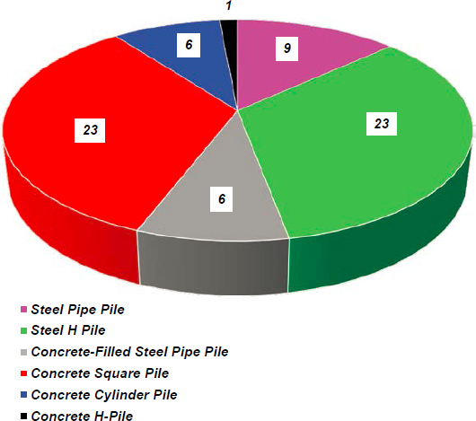
The distribution of the pile types analyzed in this study—including steel pipe, steel H, concrete-filled steel pipe, concrete square, concrete cylinder, and concrete H—is presented in Figure 2.4.1. The minimum, maximum, and average embedded length of the piles are 6.7 m, 69.5 m, and 31.1 m, respectively; whereas the minimum, maximum, and average width or diameter of the piles are 250 mm, 1,830 mm, and 458.2 mm, respectively. Information for each pile record, including the installation method, cross-sectional area, elastic modulus, strain measurement method, residual load measurement, soil layering, and available in situ and laboratory tests of the soil deposits, is provided in Table 2.4.2. For those cases where the elastic modulus of the pile was not reported by the authors, the elastic modulus was assumed based on the available information, such as the type of pile. The residual load anticipated in each pile was calculated following the methodology proposed by Fellenius (2002), described in detail below. The load transfer behavior (e.g., side resistance-relative displacement, or t-z, curves) was computed for the reported load transfer and also following correction of the estimated residual load following pile driving.
2.5 Methodology
2.5.1 Method A
The drag load acting on a pile can be estimated using the neutral plane method (Fellenius 1984) and the balance of pile forces. The proposed Method A for estimating drag load is demonstrated utilizing an example drag load calculation for a precast, prestressed concrete square pile (P17, Tables 2.4.1 and 2.4.2). The width and embedded pile length are 760 mm and 54.9 m, respectively. The pile has an internal cylindrical void with a diameter of 0.419 m. The subsurface conditions at the test site consist of layers of very soft clay, loose to dense silty sand, and medium-stiff to stiff clay.
The procedure for estimating drag load utilizing design resistance and design loads is presented in Seigel et al. (2013) and has been widely adopted in the FHWA Design and Construction of Driven Pile Foundations (Hannigan et al. 2016). The first step of the procedure is to utilize an appropriate static analysis method to estimate nominal side and end bearings. For the presented example problem, the Tomlinson (1980) and Nordlund (1979) methods were utilized to calculate resistances for plastic and granular soil layers, respectively. The next step in the Seigel et al. (2013) procedure is to determine the location of the neutral plane by plotting the unfactored permanent load plus the cumulative side resistance versus the mobilized end bearing less the cumulative side resistance. This procedure requires an estimate of the mobilized end bearing, either utilizing q-z behavior in static analysis software or from engineering judgment.
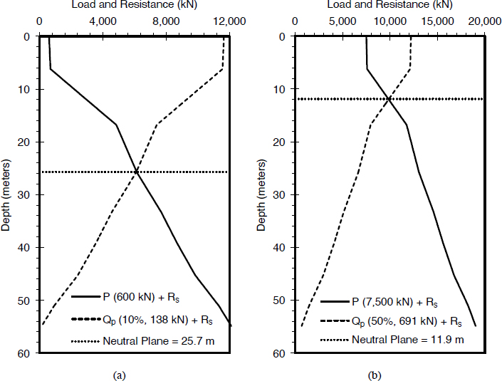
For the presented design example, two unfactored permanent loads were considered (600 kN and 7,500 kN). The corresponding mobilized end bearing for the two permanent loads were selected to be 10% (138 kN) (Figure 2.5.1a) and 50% (691 kN) (Figure 2.5.1b), respectively. The relatively small magnitude of the end bearing compared to the side resistance makes the mobilized end bearing a relatively small factor in the location of the neutral plane (e.g., if 100% toe mobilization is assumed for the 7,500 kN permanent load, the location of the neutral plane would shift less than a meter).
Using the proposed Method A, the location of the neutral plane shifts from 25.7 m to 11.9 m with the increase in permanent load. Conversely, the drag load is reduced from 5,537 kN to 2,327 kN. These values are almost certainly conservative (greater than values observed in the field) because the methodology assumes that the side resistance is fully mobilized along the length of the pile.
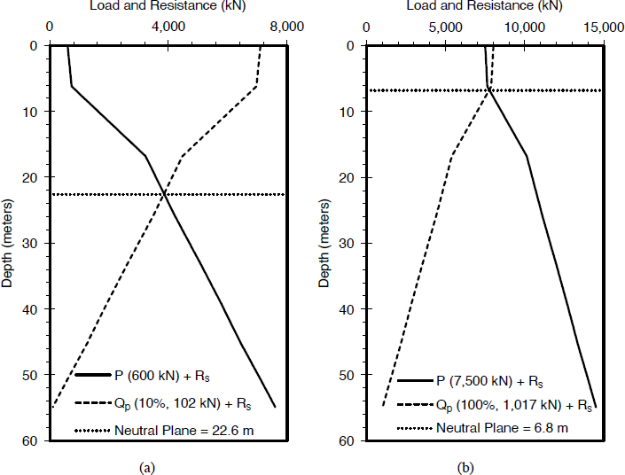
The static axial resistance methodology utilized in the Method A analysis influences the results. For instance, if the Schmertmann (1975) CPT method is used, the magnitude of drag load and the location of the neutral plane change notably. For the same two permanent loads previously considered [600 kN (Figure 2.5.2a) and 7,500 kN (Figure 2.5.2b)], the location of the neutral plane shifts from 22.6 m to 6.8 m. The assumed toe mobilization for the two load cases (600 kN and 7,500 kN) were 10% (102 kN) and 100% (1,017 kN), respectively, and were assessed based on the ratio of permanent load and ultimate side resistance. When using the Schmertmann (1975) static resistance, the drag load was reduced from 3,262 kN to 277 kN for the two permanent design loads considered.
The accuracy of the static axial resistance methodology utilized for Method A directly influences the accuracy of the Method A results (e.g., the more accurate the static axial resistance method, the more accurate the neutral plane/drag load estimate). However, even if the static resistance is determined accurately (e.g., from an instrumented load test or dynamic testing), Method A results will remain uncertain because full mobilization of side resistance is assumed. This effect can be highlighted by comparing Method A results with direct field observations.
2.5.1.1 Comparison of Method A and Field Observations
Consider the test pile from Bradshaw et al. (2012) (P1, Tables 2.4.1 and 2.4.2), the open-ended steel pipe pile had a diameter and wall thickness of 1,830 mm and 33 mm, respectively. The pile length and penetration depth of the test pile were 41.6 m and 41 m, respectively. The subsurface conditions consist of sand and gravel fill underlain by layers of gravel, sand, and nonplastic silt.
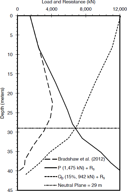
Using the Meyerhof (1976) static resistance method with the proposed Method A and a permanent load of 1,475 kN [which corresponds to the first stage of the Bradshaw et al. (2012) static loading test] with a mobilized toe-bearing resistance of 15% (942 kN), the neutral plane was determined to be 29 m as depicted in Figure 2.5.3. From the first stage of the residual, corrected static load test, the neutral plane was between 22.6 m and 26.2 m. The difference between the field-observed load distribution and the Method A distribution can be attributed to many factors. The side resistance determined from the Meyerhof (1976) resistance method exceeds the actual side resistance below about 9 m. The Meyerhof (1976) method may have overpredicted the ultimate field resistance or the discrepancy may be due to the side resistance only being partially mobilized (accounted for by the proposed Method B). A further discrepancy is due to the assumed mobilized toe-bearing resistance (15% or 942 kN) compared to the observed mobilized toe-bearing resistance (263 kN). However, even if correcting for the assumed toe-bearing resistance, the neutral plane would still be 28 m.
Perhaps the greatest difference between Method A and field-observed load distribution is the drag load. The drag load observed in the field was 2,647 kN. Conversely, the drag load determined utilizing the Method A approach was 5,317 kN (more than 100% higher than the field-observed drag load). Although conservative, the Method A approach in this example more than doubles the drag load considered for design. The robustness of the proposed Method B can correct many
of the deficiencies of Method A by explicitly considering the load transfer behavior of the pile (i.e., t-z and q-z).
2.5.1.2 Soil Settlement Profiles with Method A
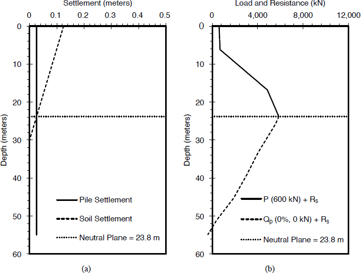
Method A can be adopted for use with a specified settlement profile by setting the neutral plane to the depth where the pile settlement is equal to the soil settlement. The pile settlement can be determined utilizing the methodology presented in Briaud and Tucker (1997). Consider an arbitrary ground surface settlement of 0.125 m, which varies linearly to zero at a depth of 30 m, developed, for example, as a result of embankment filling or liquefaction. If Pile P17 (Tables 2.4.1 and 2.4.2) experienced a permanent load of 600 kN and was subjected to the arbitrary settlement profile, the static axial resistance computed using the Tomlinson (1980) and Nordlund (1979) methods would produce an estimate of the neutral plane location of 23.8 m (Figure 2.5.4a). The neutral plane location (23.8 m) determined from the pile and soil settlement yields the load distribution depicted in Figure 2.5.4b.
Based on the pile load distribution, the drag load resulting from the soil settlement would be 5,263 kN. By contrast, the drag load calculated utilizing Method B was 826 kN (Figure 2.5.22c). As with the field comparison, Method A provides a conservative estimate of the drag load, whereas the proposed Method B provides a more reasonable estimate and is preferred for design.
Similar to how the choice of static resistance methodology influences the estimated location of the neutral plane (Figures 2.5.1 and 2.5.2), the choice of pile settlement and soil settlement methodology will influence the location of the neutral plane when utilizing soil settlement profiles with Method A.
2.5.2 Method B
2.5.2.1 Evaluation of Uncorrected Load Transfer and t-z Curves
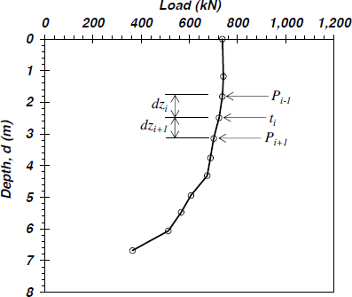
The measured load-displacement curve of the pile head and force distribution along the pile length for each load increment are used to develop the distribution of the side resistance, t, with the pile movement relative to the soil, z. First, the unfactored pile head load, P0, and pile head displacement, s, are identified from the P0-s graph for each load increment. Then the load transfer data along the embedded pile length at the instrumented depth, d, (i.e., variation in P with d) are used to calculate the elastic compression, dw, of each pile segment. The length, dzi, of each segment, i, of the pile between the strain gauges along the pile is obtained. The elastic compression of each pile segment, dwi, is then calculated using
| Equation 2.5.1 |
where Ei is the elastic modulus (which may be a composite modulus), and Ai is the cross-section area of the pile segment. The relative soil-pile displacement with respect to surrounding soil, z, is determined at each depth of the strain gauge by subtracting the total elastic compression of the pile:
| Equation 2.5.2 |
at the location of the pile segment from the pile head displacement:
| zi = s − w | Equation 2.5.3 |
where n = number of segments. This process is repeated for each pile head loading increment. The mobilized side resistance at each strain gauge level, ti, is determined from the load distribution along the pile (Figure 2.5.5) using
| Equation 2.5.4 |
where Ci = circumference of the pile corresponding to the pile segment i. The side resistance equals the ratio of the change in load in two successive strain gauges and the surface area of the pile segment between the two strain gauges. The methodology described herein is used to develop the t-z curves for each pile in the load test database (previously presented as Table 2.4.1).
2.5.2.2 Example of Uncorrected t-z Curves for Pile Types
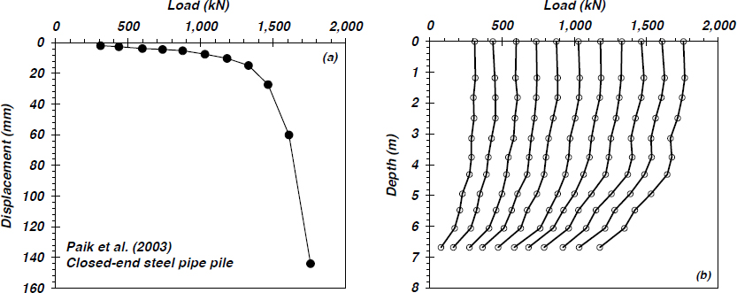
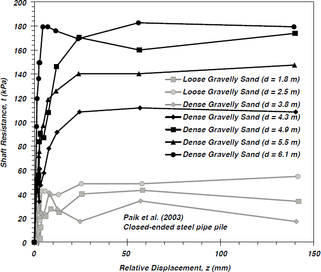
The results of a static load test on an instrumented, closed-ended steel pipe pile—including the load-displacement curve at the pile head and the load distribution along the pile length, as described by Paik et al. (2003)—are presented in Figure 2.5.6. The test pile was driven using an ICE 42-S diesel hammer at a bridge construction site in Lagrange County, Indiana, USA. The embedded length, diameter, and wall thickness of the test pile are 6.87 m, 356 mm, and 12.7 mm, respectively. The elastic modulus of the pile is 200 GPa. The details of the pile were previously provided in Tables 2.4.1 and 2.4.2 for the pile identified as P5. The subsurface conditions at the test site consist of loose gravelly sand to dense gravelly sand over the embedded length of the pile. Using the P0-s graph (Figure 2.5.6a) and P0-d graph (Figure 2.5.6b) the variation of side
resistance with the relative pile movement was determined (Figure 2.5.7) by using the methodology described above and Equations 2.5.1 to 2.5.4. The distribution of the side resistance indicates a largely plastic response with slight displacement-softening behavior in all strain gauge locations except the strain gauges located at depths of 3.8 m and 4.9 m below the ground surface, where side resistance exhibits a noticeable displacement-softening response. In general, the side resistance increases with the relative density of the soil. The maximum residual load-uncorrected side resistance in the test pile is 182.6 kPa at a corresponding z = 55.9 mm.
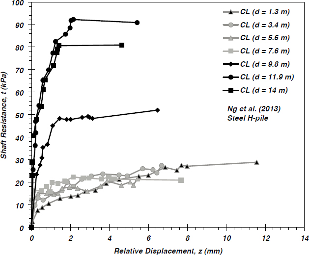
The pile head displacement and load distribution for a steel H-pile (HP 250 × 62 or HP10 × 42), designated P8 in Tables 2.4.1 and 2.4.2, driven at a test site in Clarke County, Iowa, and reported by Ng et al. (2013), are presented in Figure 2.5.8. An open-ended diesel hammer was used to drive the pile to a depth of embedment of 17.3 m. The test pile was instrumented with vibrating-wire strain gauges along the centerline of the pile along the web of the section. The details for the
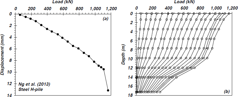
pile and the subsurface conditions are given in Tables 2.4.1 and 2.4.2, respectively, the latter of which consists of predominantly moderately overconsolidated, low-plasticity clay. Figure 2.5.9 presents the variation of side resistance with the relative soil-pile movement determined from the variation of P0 with s and P with d. The mobilized side resistance along the pile indicates displacement-hardening behavior, which could be attributed to the amount of overconsolidation of the clay layer, characterized with an OCR of 4.5. The maximum residual load-uncorrected side resistance in the test pile is 92 kPa, corresponding to z = 2.1 mm. Residual load was not measured after the pile driving; hence, the residual load was calculated to develop corrected t-z curves for this test pile, described below.
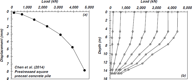
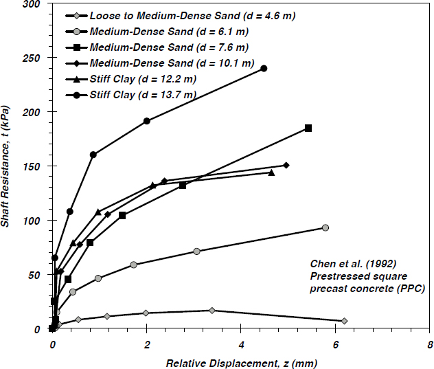
The pile head displacement and load distribution along the shaft of an instrumented, prestressed, square concrete pile (P13 in Tables 2.4.1 and 2.4.2), which was driven using an ICE I-46 open-ended diesel hammer at the Bayou Zourie bridge reconstruction site at Vernon Parish, Louisiana, and reported by Chen et al. (2014), are presented in Figure 2.5.10. The width and embedded pile length are 610 mm and 15.2 m, respectively. The test pile was instrumented with sister bar strain gauges along the embedded pile length. The subsurface conditions at the test site consist of layers of loose to medium-dense sand and silty sand with occasional pockets of clayey sand. The pile toe is located in a stiff clay layer underlying the medium-dense sand deposit. The elastic modulus of the test pile is 47 GPa, which is determined from the strain data measured during the first load increment, as reported by Chen et al. (2014). The corresponding variation of side resistance with the relative pile displacement is presented in Figure 2.5.11. The side resistance mobilized along the pile indicates displacement-hardening behavior except for the instrumented depth of 4.6 m, which exhibited displacement-softening behavior.
2.5.2.3 Evaluation of Displacement-Softening Behavior in Pile Side Resistance
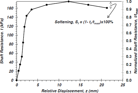
The previous discussion describing the calculation of t-z curves noted that instrumented pile segments can exhibit displacement-softening behavior where the unit side resistance may exhibit post-peak softening. An effort was therefore made to quantify the magnitude of softening and to identify factors governing softening for those instrumented pile segments exhibiting this behavior, using the back-calculated empirical t-z curves. Figure 2.5.12 shows the variation of mobilized side resistance and normalized side resistance with relative displacement for P3 (see Appendix A, Figure A3) at an instrumented depth of 13.4 m. The initial t-z response indicates a steep initial rise in mobilized side resistance to attain a maximum side resistance of tmax = 175 kPa at z = 12.3 mm. The mobilized t then reduces with z, indicating displacement-softening behavior, and reaches the final observed side resistance, tf =161 kPa, at the maximum relative displacement of zmax = 21.3 mm. The percentage softening, Sf, is calculated using Equation 2.5.5, given by
| Equation 2.5.5 |
to indicate that pile P3 exhibits a percent softening of 8% at zmax.
The quantification of displacement softening and relation to soil properties or effective stresses would serve to help guide foundation engineers in the selection of an appropriate t-z curve model in forward analysis. For example, soil-pile interfaces under low-effective confining stresses where dilative soil tendencies are expected should exhibit a greater propensity for displacement softening than those under high-effective confining stresses (and are more likely to exhibit contractive tendencies). Nonsensitive soils with higher strengths should likewise exhibit a greater tendency for displacement-softening behavior than those with lower strengths. Further, rough concrete-soil interfaces are expected to exhibit greater dilative tendency and potential for displacement softening than smoother steel-soil interfaces.
Figure 2.5.13a presents the percentage softening with vertical effective stress, , for steel and concrete piles determined from the uncorrected load transfer database (Appendix A,
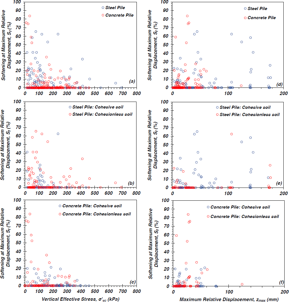
Figures A1 to A68). Many piles at low show displacement-hardening behavior indicated by Sf = 0 up to the maximum observed relative pile displacement, zmax; in contrast, one instrumented pile segment exhibits displacement-softening behavior as great as 650 kPa. No clear differences between concrete and steel pile segments can be observed. Figures 2.5.13b and 2.5.13c separate the percentage softening for steel and concrete pile segments based on their predominant location within cohesive or cohesionless soil. Although a global trend of the reduction of Sf with , may be observed, attempts to identify a correlation were unsuccessful given the extensive scatter in the dataset.
Figures 2.5.13d, 2.5.13e, and 2.5.13f present the variation of percent softening with zmax for steel and concrete pile segments within plastic and cohesionless soil. It would be expected that those pile segments in soils likely to exhibit displacement-softening behavior and experience greater relative displacement should exhibit greater magnitudes of softening. However, a clear relationship between Sf and zmax does not exist. Given that a large amount of the instrumented pile segments experienced 20 mm of relative displacement or less, the lack of an observed trend may be attributed in part to insufficient relative displacement.
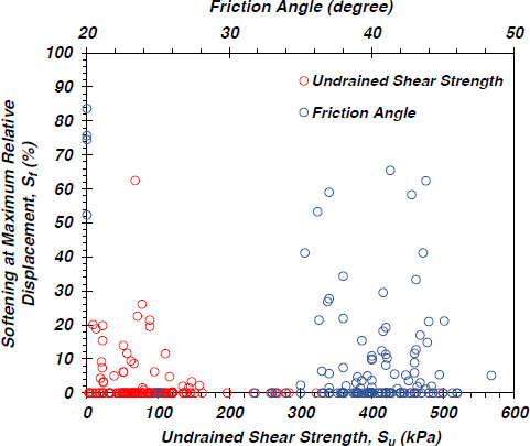
The variation of Sf with the undrained shear strength, Su, of plastic soil, and friction angle for cohesionless soil, is shown in Figure 2.5.14. For those piles exhibiting displacement-softening behavior in plastic soils, it may be observed that Sf apparently decreases with increases in Su, which is counterintuitive from the expected soil mechanics governing the soil-pile interface behavior. Likewise, no trend in Sf with the friction angle may be observed. However, numerous pile segments indicate no softening for the maximum relative displacement achieved during the static loading test, further obscuring possible trends between undrained shear strength and friction angle. Note that the Su and friction angle of the soils surrounding the instrumented pile segments are correlated from either CPT- or SPT-based measurements, and the use of these correlations necessarily introduces a large degree of uncertainty in the estimated in situ soil properties. Moreover, static loading tests are conducted after pile driving, which induces a well-known degree of disturbance, and thus changes in the soil properties in the vicinity of the pile, such that the estimated strength parameters for these soils following installation are difficult to predict (hence the use of empirical, post-installation, static pile resistance methods).
Based on the assessments described previously, it is difficult to reliably predict a priori whether or not a given pile segment will exhibit displacement-softening behavior. As such, the use of static loading tests for support of project-specific design continues to represent the best practice for efficient foundation engineering.
2.5.2.4 Evaluation of Residual Load Transfer and Residual Load-Corrected t-z Curves
Residual loads are often locked into the pile after pile driving due to the post-driving reconsolidation or recovery of the soil and/or partial unloading of the pile following the last hammer strike (Fellenius 2002). From the perspective of conditions at the soil-pile interface, residual load generally develops due to negative side resistance in the upper portions of the pile, which transitions to positive side resistance and toe-bearing resistance for points below. The residual load is necessarily generated to provide static force equilibrium in the pile. Neglecting the presence of the residual load does not influence the measured ultimate resistance of the pile (i.e., the sum of ultimate side resistance and displacement-compatible toe-bearing resistance); however, the interpretation of the load transfer along the pile shaft and at the toe may be significantly affected if the residual load distribution along the pile is ignored (Fellenius 2002). Thus, back-calculated unit side and toe-bearing resistances derived from instrumented static loading tests could be in gross error, depending on the magnitude of residual load that has developed.
The residual load was therefore calculated for each pile in the load test database using the Fellenius (2002) method. First, the load transfer distribution at the maximum test load was selected, assuming that the side resistance had been fully mobilized. Inspection of t-z curves provided previously shows that while some soil-pile interfaces exhibited nearly perfectly plastic behavior, others exhibited displacement softening and hardening. Thus, some error in the estimated residual load may be introduced by this assumption. The cumulative ultimate side resistance, Tu, was then estimated at each strain gauge location from the load transfer distribution using
| Equation 2.5.6 |
The factor of two in the denominator of Equation 2.5.6 assumes that the residual load needs to be reversed before the development of fully mobilized positive side resistance. The variation of the true cumulative side resistance, , with depth is then estimated using
| Equation 2.5.7 |
considering the effective stress-based β Method, where C = pile circumference, and = vertical effective stress. The latter quantity is calculated based on the soil properties and the groundwater conditions reported at the corresponding test site (see Table 2.4.2). Where the unit weight of a particular stratum was not reported, it was estimated from the available correlations to in situ measurements (e.g., CPTs, SPTs) or available laboratory data (see Section 2.2) to obtain an effective stress, and this effective stress was used in Equation 2.5.7. Given the variation of with depth and C, the β coefficient necessary to match with that measured (i.e., Tu) along the upper part of the pile is determined. The estimated true pile load, P*, at each strain gauge location is then calculated by subtracting from the applied head load, P0:
| P*= P0 − | Equation 2.5.8 |
The estimated distribution of the residual load, Pr, with depth is then calculated by subtracting the measured pile load at each strain gauge location from P*:
| Pr = P0 − P* | Equation 2.5.9 |
The results of an instrumented steel H-pile (P8 in Tables 2.4.1 and 2.4.2), including the distributions of Tu, , P*, and Pr, are shown in Figure 2.5.15a. The maximum residual load is 302 kN, occurring at a depth of 14 m, identified by the depth at which the polarity of the Pr curve reverses and is associated with the transition from negative side resistance to positive side resistance. Figure 2.5.15b presents the resulting residual load-corrected load transfer distribution; the measured toe-bearing resistance increased following correction for the residual load (i.e., from 296 to 558 kN for the last load increment). The shape of the load transfer distribution is noticeably impacted by the residual load correction and indicates that the actual estimated side resistance is smaller than that computed prior to correction (Figure 2.5.15a). Inspection of Figure 2.5.15b indicates that the neutral plane arising from the residual load is located at a
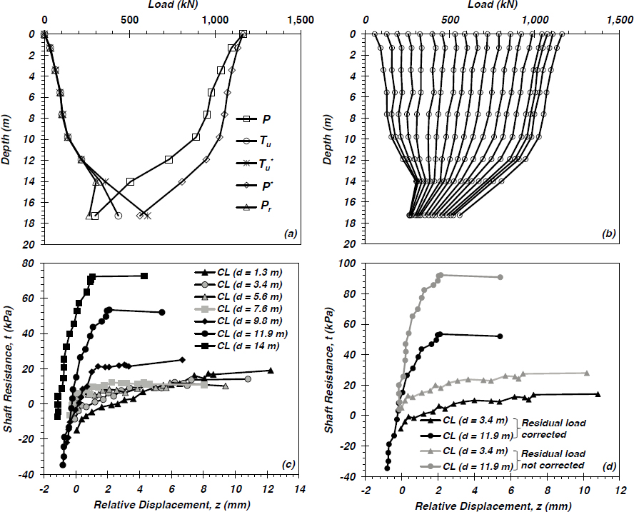
depth in close proximity to the instrumented depth of 14 m. Figure 2.5.15c presents the variation of residual load-corrected t-z curves for different instrumented depths of the pile; the t-z curves for the segments above the neutral plane initiate at noticeably negative side resistances, whereas the t-z curve for the depth of 14 m exhibits largely positive side resistance for the entirety of the static loading test. The effect of residual load correction on the t-z curves is compared directly in Figure 2.5.15d; the residual load correction results in a decrease in side resistance (selected instrumented depths correspond to 3.4 m and 11.9 m). For example, the maximum side resistance before and after residual load correction at the depth of 11.9 m is 92 and 53 kPa, respectively.
The results of an instrumented, prestressed square concrete pile, including the distribution of P, Tu, , P*, and Pr, are presented in Figure 2.5.16a. No neutral plane developed because the
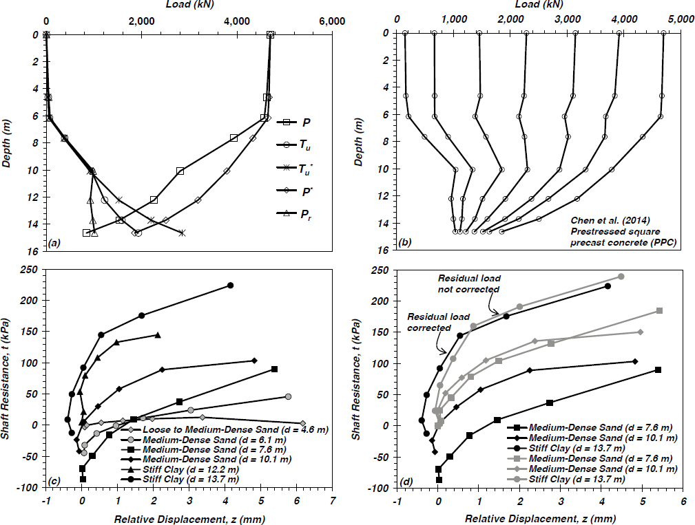
mobilized side resistance exhibited displacement-hardening behavior (Figure 2.5.11), and the maximum side resistance was not fully mobilized. The maximum residual load was 1,011 kN occurring at the toe of the pile (i.e., a depth of 15.2 m). As shown in Figure 2.5.16b, the corrected load transfer distribution indicates that a pile head load of approximately 2,250 kN was necessary to overcome all of the negative side resistance that had developed following installation. The residual load-corrected t-z curves for the various instrumented depths of the pile are presented in Figure 2.5.16c; note that those corrected t-z curves with a minor (e.g., 0.5 mm or less) amount of initial negative relative soil-pile movement, z, reflect potential error in the Young’s modulus of the pile and may be considered effectively zero. This can be appreciated through the comparison of Figures 2.5.15c and 2.5.16c, for which a significantly larger initial t-z response may be observed in the H-pile (with reliable Young’s modulus, presented in Figure 2.5.15c). The t-z curves with and without residual load correction are compared in Figure 2.5.16d. The maximum side resistance at the instrumented depth of 7.6 m without and with residual load correction equals 185 and 90 kPa, respectively, a reduction of approximately one-half, due to its position in the upper half of the pile. In contrast, the maximum side resistance at the instrumented depth of 13.7 m without and with residual load correction equals 239 and 224 kPa, respectively; the smaller margin reflects its deeper location where the effects of the residual load on side resistance are smaller.
2.5.2.5 Database of Uncorrected and Residual Load-Corrected Load Transfer and t-z Curves
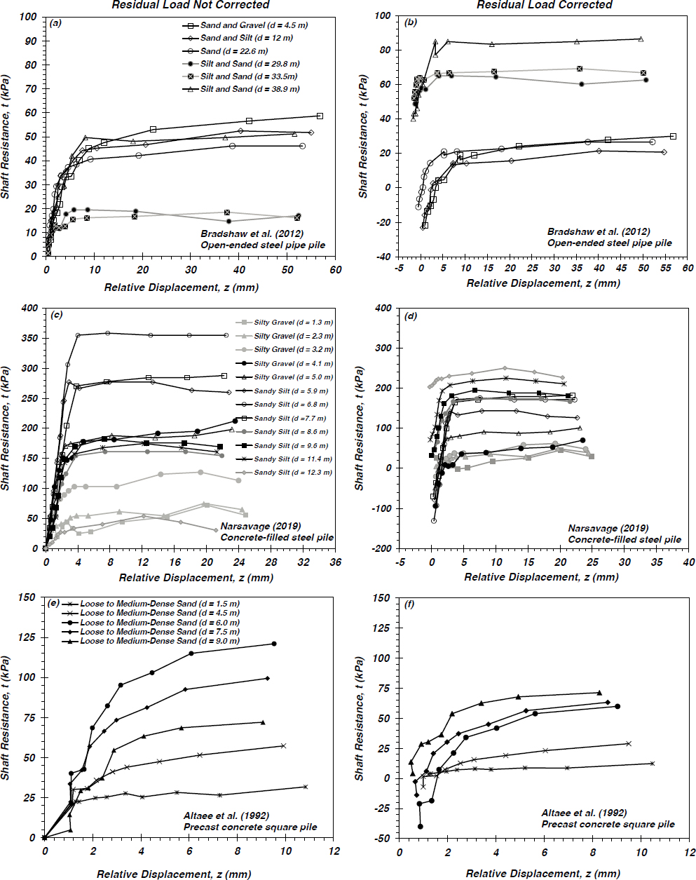
The procedure described above was implemented for all the piles in the load test database to develop uncorrected and residual load-corrected t-z curves. Examples of the effect of the estimated residual loads on the t-z curves for various pile types in the load test database, including an open-ended steel pipe, concrete-filled steel pipe, and precast concrete square piles are presented in Figure 2.5.17. The details of these three pile records are reported in Tables 2.4.1 and 2.4.2. In each case, the unit side resistance was significantly impacted following correction for the residual load; however, the impact varied as a function of the degree of side resistance mobilized following installation and before static load testing. For the case of the precast square concrete pile, all of the t-z curves exhibited lower side resistance following correction when compared with the uncorrected t-z curves.
2.5.2.6 Evaluation of Pile Unit Toe-Bearing Resistance
Application of the load transfer modeling approach to estimate the relationships between mobilized toe and side resistance and pile head displacement requires that the variation of the unit toe-bearing resistance with toe displacement be known or estimated. In general, strain gauges are provided some distance above the pile toe to mitigate the potential installation-induced damage. Hence, the true toe-bearing resistance of a given pile is generally unknown. For each pile, the toe-bearing resistance was estimated using linear extrapolation of the load transfer data from the last two strain gauge depths to the depth corresponding to the pile toe. The unit toe-bearing resistance, q, is determined by dividing the extrapolated toe-bearing resistance by area of the pile toe. For the cases of open- and closed-ended pipe piles, open-ended cylinder piles, and precast concrete square piles, the full basal area was used to determine the unit toe-bearing resistance of the pile. In contrast, the unit toe-bearing resistance of steel H-piles was computed using the ICP Method (Jardine et al. 2005), where the H-pile base area, Ab, is calculated considering the pile steel area, As, and its dimensions, using
| Ab = As + 2 * Xp (D − 2t) | Equation 2.5.10 |
where
| Equation 2.5.11 |
if B/2 < (D − 2t) < B, and
| Equation 2.5.12 |
if (D − 2t) > B, where D = depth; t = thickness; and B = width of flange.
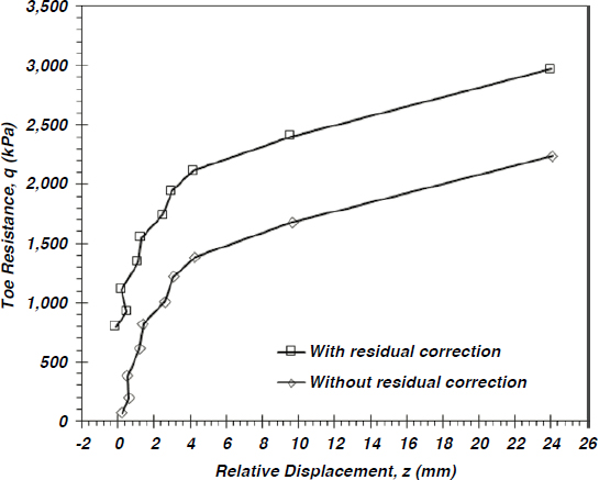
Once the unit toe-bearing resistance is calculated for each pile head load increment, the toe-bearing displacement, z, is calculated for each increment by subtracting the total elastic shortening of the pile from the measured pile head displacement for that increment. Figure 2.5.18 presents an example of the variation of the unit toe-bearing resistance with toe displacement for a concrete-filled, closed-ended steel pipe pile without residual load correction and with residual load correction. Figures 2.5.15a and 2.5.16a show that the toe load of an instrumented pile generally increases following the correction for residual load. The comparison of the calculated q-z curves for the case with and without residual load correction is shown in Figure 2.5.18, indicating a larger mobilized toe-bearing resistance for the case of residual load correction.
The pile head load-displacement, load transfer, and calculated mobilized unit side and toe-bearing resistance curves—each with and without residual load correction—determined for each pile in the load test database are provided in Appendix A. The database will be used to verify the accuracy of various t-z models available to foundation engineers to design piles in view of displacement performance and resistance. Furthermore, the deployment of a consistent,
statistically rigorous evaluation of the selected t-z curve models described in Section 2.3 will lend increased confidence to foundation engineers wishing to use Method B to estimate drag loads.
2.5.2.7 Simulation of Load Transfer and Drag Load Using Software
Two alternative methods to estimate the drag load of driven piles developed as a result of consolidation or liquefaction-induced settlement are proposed. Whereas Method A assumes that all positive and negative side resistance is fully mobilized when locating the neutral plane, the use of load transfer modeling (i.e., Method B) allows this assumption to be relaxed. The net result, particularly for displacement-softening and displacement-hardening soil-pile interface responses, is that the drag load may be reduced given that the amount of local settlement at a particular depth is used to directly estimate negative and positive side resistance. The drag load may be reduced considerably for long piles, where the amount of total displacement is relatively small (on the order of several inches), and where full mobilization of side resistance is not likely to occur over the full length of the pile.
The software package TZPILE (Ensoft 2021) was used to illustrate the methodology for Method B, which allows the simulation of pile head displacement and load transfer considering pile material and geometrical characteristics and the empirical (i.e., back-calculated) t-z and q-z curves as an input. Note that any software package that facilitates the specification of t-z curves and soil settlement profiles can be used to conduct the analyses described below (e.g., RSPile, APILE, UniPile, TZPILE, etc.); furthermore, the use of TZPILE in this study shall not be interpreted as an endorsement of the software by the authors or TRB.
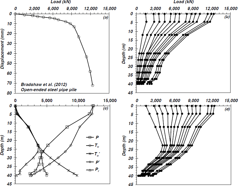
The pile head displacement and load transfer distribution along the shaft of an instrumented open-ended steel pipe pile (P1), installed using an ICE-66 80 vibratory hammer in Rhode Island and reported by Bradshaw et al. (2012) are presented in Figures 2.5.19a and 2.5.19b. The outer diameter and embedded pile length are 1,830 mm and 41 m, respectively. The wall thickness of the steel pile was 33 mm. The test pile was instrumented with sister bar strain gauges along the embedded pile length. The subsurface conditions at the test site consist of layers of sand and gravel with nonplastic silt. Based on the results shown in Figures 2.5.19c and 2.5.19d, the maximum post-installation residual load exceeded 3,000 kN, the result of which significantly impacted the true load transfer distribution.
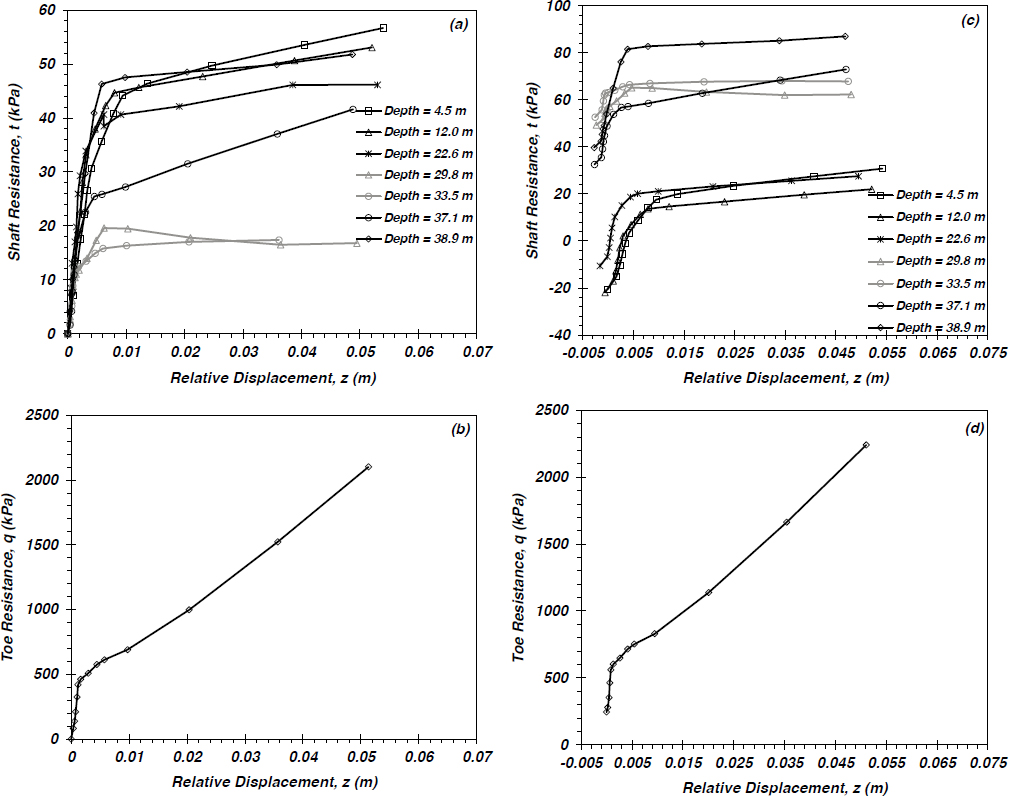
The variation of the mobilized side and unit toe-bearing resistance with the relative pile movement determined directly from the static loading test results (i.e., no correction for residual load) are displayed in Figures 2.5.20a and 2.5.20b, respectively. The unit end bearing of the pile was determined by assuming that the toe acted in a fully plugged condition during the relatively slow static loading test. This is in contrast to how the pile may act during installation depending on the inertial response of the plug due to the impact or vibratory acceleration and corresponding stress waves. The mobilized unit side resistance indicates displacement-hardening behavior except for the instrumented depth of 29.8 m, which exhibits displacement softening. The residual load-corrected t-z and q-z curves for this pile, determined using the effective stress approach described previously, are presented in Figure 2.5.20c and Figure 2.5.20d, respectively.
The results of the instrumented static loading test that were previously summarized graphically in Figure 2.5.19 were simulated using TZPILE for the uncorrected and residual load-corrected scenarios to demonstrate the effectiveness of the proposed Method B for the assessment of the drag load. For the first case where residual load is not explicitly considered, the uncorrected t-z and q-z curves are used as input to the TZPILE program. A comparison of the pile head load-displacement curve for the simulated and measured responses is presented in Figure 2.5.21a. The simulated response is in excellent agreement with the measured response to a pile head load. The simulated load transfer distribution is shown alongside the load transfer distribution obtained from the instrumented static pile loading test in Figure 2.5.21b. Although some minor
differences may be noted, the load transfer is more or less accurately captured for pile head loads for all depths and accurately captured below a depth of about 5 m. It should be noted that the upper portions of piles are often subjected to or exhibit flexure during static loading tests due to slight misalignment of the hydraulic jack(s) and/or differential mobilization of the side resistance from the reaction piles. Such experimental errors are expected to accumulate at the later stages of static loading tests, which likely serves to explain, in part, some of the noted differences between the measured and computed load transfer and pile head load-displacement responses.
A comparison of pile head displacement between the simulated and measured response of the same pile, but now in consideration of the residual load that existed prior to static loading and estimated using the Fellenius (2002) approach, is presented in Figure 2.5.21c and Figure 2.5.21d. Due to the lack of convergence of the numerical simulation within the software package TZPILE, the head load below 6,000 kN cannot be simulated for this case. The simulated response agrees with the measured response for the loads for which a solution was obtained. The load transfer graphs determined from the in situ tests are compared with the TZPILE simulation in Figure 2.5.21b. Simulated load transfer graphs considering residual load correction are in very good agreement with the measured response.
2.5.2.8 Simulation of Drag Load Using Load Transfer Software
The proposed Method B for estimating drag load in settling soils using the load transfer approach is demonstrated through an example of drag load simulation of a precast, prestressed concrete square pile (P17, Tables 2.4.1 and 2.4.2). The width and embedded pile length are 760 mm and 54.9 m, respectively. The pile has an internal cylindrical void with a diameter of 0.419 m. The test pile was instrumented with sister bar strain gauges along the pile length. The subsurface conditions at the test site consist of layers of very soft clay, loose to dense silty sand, and medium-stiff to stiff clay. The in situ load-displacement curve, the load transfer distribution, the load transfer distribution adjusted to account for the estimated residual load, and the uncorrected and residual load-corrected t-z and q-z curves are presented in Figure A17 (Appendix A).
The software package TZPILE was used to simulate the pile head load-displacement behavior and load transfer distribution using the back-calculated t-z (Figures A17c and A17e) and
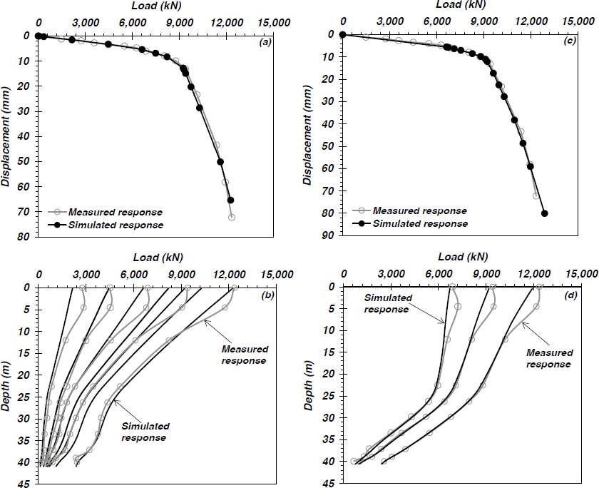
q-z curves (Figure A17f). The actual pile properties presented in Tables 2.4.1 and 2.4.2 were also used as input for this analysis. To simulate the development of drag load within the pile as a result of downward soil movement (i.e., settlement) adjacent to the pile, an arbitrary settlement profile was specified in the analysis: the settlement of the ground surface was set to 0.125 m (approximately 5 inches) decreasing linearly to 0 m at a depth of 30 m. Note that the software allows for the specification of any settlement profile and that any number of analyses can be conducted to evaluate the time-rate of drag load development if the corresponding time-varying settlement profiles have been computed as part of a project. The analysis was completed for two cases: one case assuming that no residual load exists and a second case recognizing that the residual load exists and must be included to correctly capture the side and toe-bearing resistance.
The measured and simulated pile head load-displacement and load transfer distribution for the case without residual load for the selected pile are presented in Figures 2.5.22a and 2.5.22b. Similarly, with consideration of the residual load in the pile, the simulated response also shows good agreement with the measured response. The results of the drag load simulation again consider a ground surface settlement of 0.125 m varying linearly to zero at 30 m (Figure 2.5.22c). The drag load is clearly apparent in Figure 2.5.22c for the applied pile head load of 600 kN; the load increases with depth to the neutral plane, corresponding to the reversal from negative
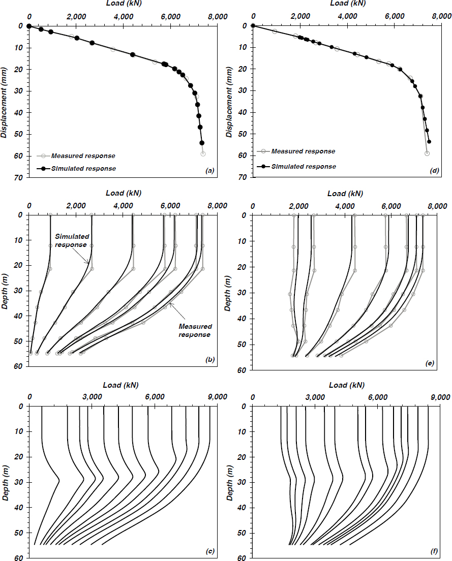
to positive side resistance and occurring just above 30 m to a maximum of 1,426 kN. The difference between the load at the neutral plane and the pile head, 826 kN, is the drag load due to downward soil settlement. For the same example analyzed utilizing Method A, the predicted neutral plane and drag load were 23.8 and 5,263 kN (six times the Method B predicted drag load), respectively. As previously discussed, Method A provides overly conservative estimates of drag load due to assuming full mobilization of side resistance.
As additional loading is placed on the pile head, the neutral plane moves up, and the drag load reduces since the pile compresses elastically and moves down relative to the soil surrounding it. The drag load has been nearly eliminated for the pile head load of 7,500 kN and clearly no longer exists at the geotechnical strength limit state when all side resistance is positive and fully mobilized.
The results of the load transfer simulation for the case considering the post-installation residual load are shown in Figures 2.5.22d through 2.5.22f. The residual load-corrected load transfer is well-captured using the residual load-corrected t-z and q-z curves (Figure 2.5.22e), as is the resulting pile head load-displacement curve (Figure 2.5.22d). Considering the application of the arbitrary settlement profile, notable differences exist between this case (Figure 2.5.22f) and the case without residual load (Figure 2.5.22c). First, the load transfer distribution is more complex due to the preexisting residual load, and the neutral plane lies at a depth of 47 m. Noting that the drag load is equal to the difference between the maximum load in the pile and the load at the pile head, the drag load for the first simulated pile head load is 570 kN, approximately 30% smaller than that calculated for the case without residual load. As additional loads are placed on the pile head, the neutral plane shifts from 47 m to approximately 29 m, as a consequence of the deeper loads exceeding the residual load in the pile. Further loading results in continuing upward movement of the neutral plane until a load of approximately 7,450 kN, when the drag load is nearly eliminated. It is observed that consideration of the residual load resulted in the computation of a smaller drag load since all aspects of the actual loading within the pile were considered and accounted for in the load transfer simulations.
2.6 Comments on Seismically Induced Downdrag and Drag Load
Proposed revisions to the specifications for consideration by AASHTO address the occurrence of downdrag and the resulting drag loads arising from the dissipation of excess pore pressure generated during a seismic event and the corresponding reconsolidation settlement. It is critical to recognize that (1) generation and dissipation of excess pore pressure will lead to local volumetric strain and thus settlement, and (2) excess pore pressures can and will be generated in plastic soils, which are not susceptible to liquefaction if the intensity and duration of loading are sufficiently large. In other words, the consequence of excess pore pressures being generated during an earthquake must be assessed for all soils within a given soil profile.
For the proposed revisions, liquefaction may be defined as “the transient or sustained loss of shear stiffness and strength in a saturated, liquefaction-susceptible soil due to the generation of excess pore pressure.” Likewise, cyclic softening may be defined as “the partial degradation in shear stiffness and strength of nonliquefaction-susceptible soils due to excess pore pressure generation.” Although it is well-recognized that soils susceptible to liquefaction will exhibit reconsolidation strains and the corresponding settlements following the generation of excess pore pressure, it is less widely recognized that soils susceptible to cyclic softening will also exhibit post-seismic settlements upon excess pore pressure dissipation. The following discussion addresses liquefaction susceptibility, liquefaction triggering and cyclic softening, and how reconsolidation strains can be estimated.
2.6.1 Liquefaction Susceptibility
The design engineer must decide how to judge liquefaction susceptibility, which may include selection of a threshold CPT-based soil behavior type index, Ic, or by comparing stratigraphic units and the results of laboratory tests from samples retrieved from nearby borings, or both (the preferred methodology). For CPT-based liquefaction-triggering analyses, it is common to select a threshold, Ic, for which soil is assumed to be susceptible to liquefaction. Historically (Youd and Idriss 2001; Zhang et al. 2002), the threshold suggested for use in identifying liquefaction-susceptible soils has been Ic < 2.6, with caution given that soils with Ic ≥ 2.6 can often be sampled in an intact state and, as such, should be sampled for cyclic laboratory testing and assessment of the potential for liquefaction or cyclic softening under seismic loading and corresponding volumetric strain potential. It is increasingly recognized that Ic = 2.6 represents the median of a statistical distribution of Ic for which soils should be screened for liquefaction susceptibility (Stuedlein, Alemu et al. 2023). Thus, it is recommended that CPTs be paired with nearby boreholes so samples can be inspected and tested in the laboratory to develop site-specific fines content-Ic correlations and select appropriate Ic thresholds for use with liquefaction-triggering analyses and the consequences of liquefaction (e.g., reconsolidation settlement). It is also critical to recognize that determining that a soil deposit is not susceptible to liquefaction requires that an assessment of cyclic softening be conducted. Discussions of contemporary views and recent research on the subject of liquefaction susceptibility were presented at a workshop sponsored by the Pacific Earthquake Engineering Research Center in September 2022 and are described in Stuedlein, Alemu et al. (2023).
2.6.2 Liquefaction Triggering and Cyclic Softening
Numerous methods for assessing liquefaction triggering using SPT, CPT, dynamic cone penetrometer tests, and shear wave velocity measurements are available. In performing a liquefaction-triggering analysis, it is critical to understand the basis for model development, including the types of soils represented in the source databases and the modeling decisions made during model development. Different models exhibit differing magnitudes of epistemic uncertainty (Franke and Olson 2021) and associate deterministic outcomes of liquefaction triggering with differing probabilities of liquefaction triggering. The cyclic resistance of transitional soils (silty sands, clayey sands, sandy silts, low-plasticity clayey silts, etc.), which exhibit complete, though usually transient, loss of stiffness (i.e., liquefaction) under cyclic or dynamic loading is often not well-estimated using in situ penetration test correlations owing to their frequent underrepresentation in source databases (Dadashiserej et al. 2024) and the effects of partial drainage during penetration. Likewise, no shear wave velocity-based method for estimating cyclic resistance exists for transitional soils. These soils also tend to exhibit cyclic resistances, which are larger than those computed using in situ penetration test results and can be sampled and tested following best practices (e.g., mud-rotary drilling, sharpened stainless steel sample tubes) (Wijewickreme et al. 2019; Stuedlein, Dadashiserej et al. 2023) as recommended by numerous researchers (Boulanger and Idriss 2006, 2008; Bray and Sancio 2006, 2008; Wijewickreme et al. 2019; Stuedlein, Dadashiserej et al. 2023). Models to estimate the cyclic resistance of transitional soils have been proposed by Dadashiserej et al. (2024) if site-specific cyclic test data are not available.
Those plastic soils that exhibit normal consolidation lines that are parallel to their corresponding critical state lines (i.e., materials that exhibit strength normalization, typically those with a plasticity index larger than 12 to 20 depending on soil fabric, mineralogy, and other factors) are generally not susceptible to liquefaction but rather are susceptible to cyclic softening. Dadashiserej et al. (2024) demonstrated that the cyclic resistance of such soils can be reliably estimated using the SHANSEP approach proposed by Boulanger and Idriss (2007) when using
overconsolidation ratios developed from laboratory-determined preconsolidation stresses. Thus, care must be taken to determine the preconsolidation stress and corresponding overconsolidation ratio of these soils for the purposes of cyclic resistance estimation.
2.6.3 Estimation of Post-Seismic Settlements
The magnitude of post-seismic settlement is directly related to the magnitude of excess pore pressures generated during shaking. In practice, the estimate of post-liquefaction reconsolidation settlement for liquefaction-susceptible soils is commonly linked to the factor of safety against liquefaction triggering, FSL (e.g., Yoshimine et al. 2006). Deterministic liquefaction-triggering models commonly relate initial liquefaction to an excess pore pressure ratio of 100% (and/or cyclic shear strain of 3%) corresponding to FSL = 1.0. However, it is critical to recognize that FSL > 1.0 does not mean that excess pore pressures will not have been generated under strong ground motion. Volumetric strains can accumulate within a soil deposit for FSL up to 2.0 as excess pore pressures generated during shaking, which are smaller than the initial vertical effective stress dissipate. Thus, seismic design scenario-based liquefaction-triggering calculations that indicate that liquefaction will not be triggered (i.e., FSL > 1.0) do not justify the omission of reconsolidation settlement when considering drag loads or other adverse effects to transportation infrastructure.
The amount of data available for volumetric strains in transitional soils or cyclic softening-susceptible soils are much smaller than that of clean sands. Accordingly, there are no widely accepted design methods linking the factor of safety against cyclic softening to post-cyclic reconsolidation strain. The best approach for quantifying the relationship between cyclic loading, excess pore pressure generation, and post-cyclic volumetric strain of cyclic softening-susceptible soil is to perform intact sampling and cyclic and post-cyclic testing. In the absence of site-specific cyclic and post-cyclic test data, prior post-cyclic test results can be referenced and linked to the cyclic shear strains or excess pore pressures expected under a given seismic event. Such data should be based on cyclic tests performed on intact specimens (e.g., Wijewickreme and Sanin 2010; Wijewickreme et al. 2019; Verma 2019; Beyzaei et al. 2018; Jana and Stuedlein 2021; Dadashiserej et al. 2022; Sorenson et al. 2023), since the relationship between shear strain or excess pore pressure and post-cyclic volumetric strain is soil fabric-dependent, and thus reconstituted specimens will not provide an appropriate indication of the anticipated volumetric strain.
Cyclic shear strains can be estimated using nonlinear total stress site response analyses. It is typically more difficult to predict excess pore pressures, which are expected to be generated during a design earthquake. Separately, plastic soils will tend to exhibit greater post-cyclic volumetric strain for a given magnitude of excess pore pressure than clean sands owing to their greater compressibility. However, the magnitude of shear strain for a given magnitude of excess pore pressure is typically larger for plastic soils than clean sands (i.e., a plastic soil deposit will require greater shear strain than a nonplastic soil deposit to achieve the same excess pore pressure). Until a standard-of-practice method for linking the factor of safety against cyclic softening to post-cyclic volumetric strain is available, it appears reasonable to perform assessments of post-shaking reconsolidation strain for plastic soil deposits in which a factor of safety against cyclic softening (or more generally, cyclic failure) less than 2.0 is computed in alignment with post-liquefaction reconsolidation strain calculations.


