Practices for Operational Traffic Simulation Models (2025)
Chapter: 2 Literature Review
CHAPTER 2
Literature Review
This chapter presents the results of the literature review for operational traffic simulation models. Sources compiled for the literature review include guidance documents (general and DOT-specific), research reports, journal articles, and other resources. The chapter is organized into the following sections: FHWA Resources for Operational Traffic Simulation Models, Transportation System Simulation Manual (TSSM), DOT Resources for Operational Traffic Simulation Models, and Research Studies on Operational Traffic Simulation Models. Tabular summaries of literature and guidance for operational traffic simulation models are provided in Appendix D.
FHWA Resources for Operational Traffic Simulation Models
FHWA provides various resources and tools related to operational traffic simulation models, including the Traffic Analysis Toolbox (TAT), guides, and case studies. These resources are described in the following sections.
Traffic Analysis Toolbox
Traffic Analysis Toolbox 2004
The Traffic Analysis Tools Primer (Volume I of the 2004 TAT) describes the strengths and limitations of the Highway Capacity Manual (HCM) and simulation tools and provides guidance on selecting the most suitable traffic analysis tool for a given situation (Alexiadis et al. 2004). According to the primer, simulation tools can effectively assess different stages of traffic congestion and incorporate different driver and vehicle characteristics. However, the primer notes that simulation tools are data intensive and are not designed to model some situations (e.g., the effects of driveway access or on-street parking).
Volume III of the 2004 TAT provides guidance on the use of traffic microsimulation modeling software (Dowling et al. 2004). These guidelines outline a seven-step process for microsimulation modeling: (1) scoping, (2) data collection, (3) development of a base model, (4) checking for errors, (5) a comparison of model measures of effectiveness (MOEs) to field observations, (6) analysis of alternatives, and (7) final reporting. Example problems are provided for each step. Volume IV of the TAT provides specific guidance for the use of CORSIM software for microsimulation (Holm et al. 2007).
Traffic Analysis Toolbox 2019
FHWA updated Volume III of the TAT in 2019 to include more detailed guidance on data collection analysis, model calibration, and analysis of alternatives, along with a complete case study for analysis of work zone alternatives (Wunderlich et al. 2019). The 2019 guidance
(Wunderlich et al. 2019) also suggests the use of cluster analysis for the identification of travel conditions and indicates that only key performance measures should be calibrated. Figure 3 is a flowchart of the modeling process from the 2019 TAT guidance.
The updated guidelines in the 2019 TAT (Volume III) were developed to support the following objectives:
- Improve the time-dynamic representation of congestion and bottlenecks. Standard practice was highly focused on fixed or average demand patterns, resulting in unrealistic development and dissipation of congestion over time.
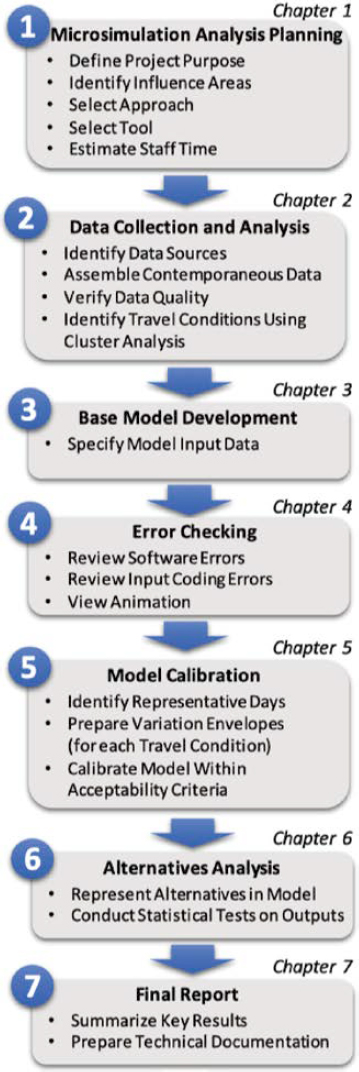
Figure 3. Microsimulation modeling process from 2019 TAT guidance.
- Incorporate consideration of non-recurrent conditions. Standard practice was to select a representative day (i.e., representative of typical recurrent congestion patterns) without consideration of incidents, weather, and other variations in travel demand.
- Remove subjective calibration criteria. Commonly used guidelines had previously indicated that calibration should be done “to the analyst’s satisfaction.” This update was intended to focus on a data-driven process based on objective criteria.
To accomplish these objectives, the updated guidelines recommend a cluster analysis of time-dependent network data (i.e., demand, weather, incidents, transit, freight, bottleneck throughput, and travel time) covering numerous days in order to detect clusters of representative travel conditions using common clustering techniques such as K-means, hierarchical clustering, and expectation maximization (Wunderlich et al. 2019). Examples of the compiled data and the clustering process are shown in Figure 4 and Figure 5.
Once clusters are identified, the guidelines recommend calibrating a single simulation seed to one representative day within each cluster that represents a distinct travel condition. It is recommended that a single day of data be used in calibrating each travel condition, as opposed to a synthetic day that is based on averages of multiple days of data. Therefore, if three distinct travel conditions were determined from the cluster analysis, three representative days would be selected for model calibration, and the process would be repeated for each representative day.
Once a representative day is selected, calibration data should be prepared. The guidance suggests that at least one measure should be related to travel times or speed profiles and that a second should be related to bottleneck dynamics (either throughput or duration). Once the data are collected, time variation envelopes are developed for each calibration dataset to represent 95% of the observed variation (∼2 sigma band) and ∼67% of the observed variation or a single standard deviation away from the mean (1 sigma band). An example of these variation envelopes is shown in Figure 6.
These bands are to be used to evaluate the model’s accuracy against field conditions following four criteria. “All four criteria should be satisfied individually for each key measure and travel condition in a single model run” (Wunderlich et al. 2019). A sample output from calibration of the first criterion is demonstrated in Figure 7.
- Criterion 1: 95% of simulated outputs fall within the ∼2 sigma band
- Criterion 2: Two-thirds of simulated outputs (and all critical time intervals) fall within 1 sigma band
- Criterion 3: Variation between model results and the representative day is less than or equal to variations within all days associated with the travel condition or cluster (calculated through the bounded dynamic absolute error)
- Criterion 4: Similar to criterion 3, but uses average simulated error (not absolute error) and is intended to flag excessive over- or underestimators
The approach presented in the 2019 TAT addresses several shortcomings of common microsimulation calibration procedures and may result in more robust calibration of models. However, this new approach requires a greater amount of data collection and data preparation and introduces statistical methods not commonly used in practice. For these reasons, the state DOT resources published after 2019 typically reference this guidance as an option when a project warrants additional data collection. For example, the Colorado DOT (CDOT) references both the 2004 and 2019 versions of the TAT (Dowling et al. 2004; Wunderlich et al. 2019) and states that smaller projects with minimal variations in travel conditions are permitted to use the 2004 microsimulation methodology (CDOT 2023). Similarly, the Kentucky Transportation Cabinet states that the 2019 version requires a larger investment in data collection and modeling, and many Kentucky projects do not require that level of effort to achieve the desired level of accuracy (Kentucky Transportation Cabinet 2021). DOT resources for operational traffic simulation models are discussed in greater detail later in this chapter.

Figure 4. Example of data assembled for travel conditions identification.
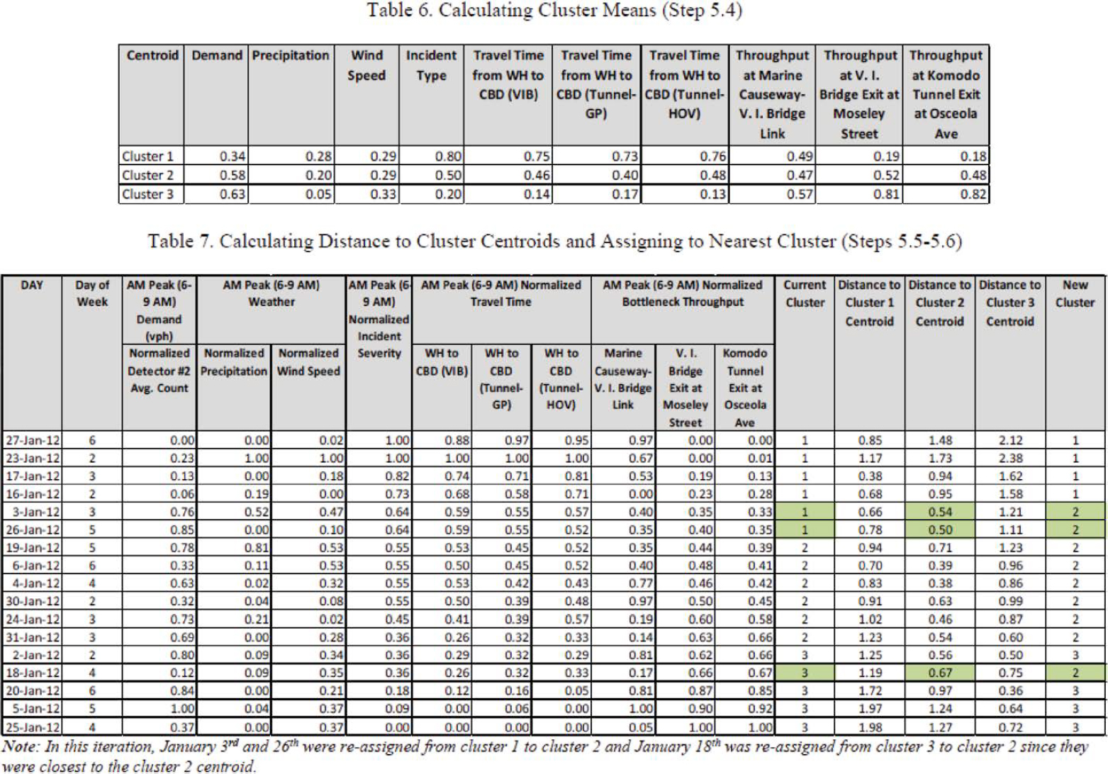
Figure 5. Example of calculating clusters and assigning days to nearest cluster.
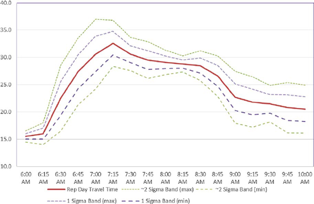
Figure 6. Example of variation envelopes for travel times.
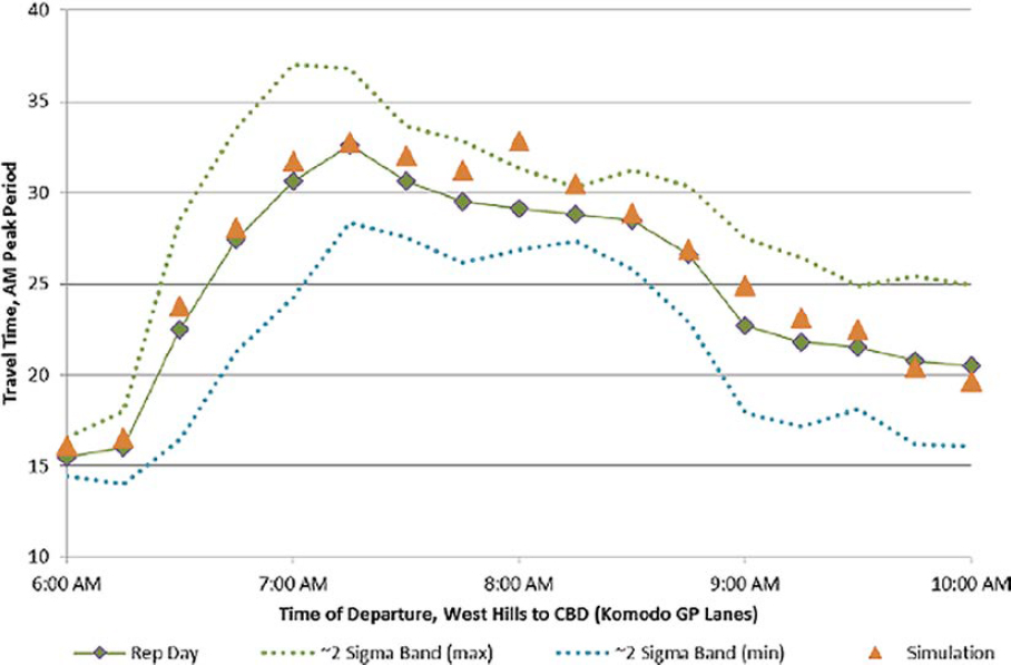
Figure 7. Example of assessing criterion 1.
Other FHWA Resources
A guidebook, case studies document, and state of the practice and gaps analysis report on MRM are also available from FHWA. The guidebook builds upon FHWA’s existing seven-step simulation methodology, offering a detailed process for MRM analysis (Hadi et al. 2022a). The case studies document on MRM focuses on technical challenges and covers three projects: downtown West Palm Beach, Florida; the Phoenix metropolitan area; and I-95 in Maryland (Hadi et al. 2022b). Example practices noted in the case examples include use of the lower-resolution models to generate the microscopic simulation model, use of demand to capacity ratio, and incorporation of open-source tools. The state of the practice and gaps analysis report reviews MRM terminology, tools, and literature, and summarizes results from teleconferences that were held with 19 agencies and companies interested in MRM (Zhou et al. 2021). The report also identifies challenges faced by agencies in incorporating MRM into their modeling practices, such as fidelity at model boundaries and training needs.
An FHWA case study on connected and automated vehicles (CAVs) used simulation modeling to evaluate the effectiveness of three CAV strategies (cooperative adaptive cruise control, speed harmonization, and cooperative merge) and a managed-lane infrastructure application on a 13-mile segment of I-66 in Northern Virginia (Ma et al. 2021). Results indicated that the CAV strategies and managed lane application helped improve traffic performance.
Transportation System Simulation Manual
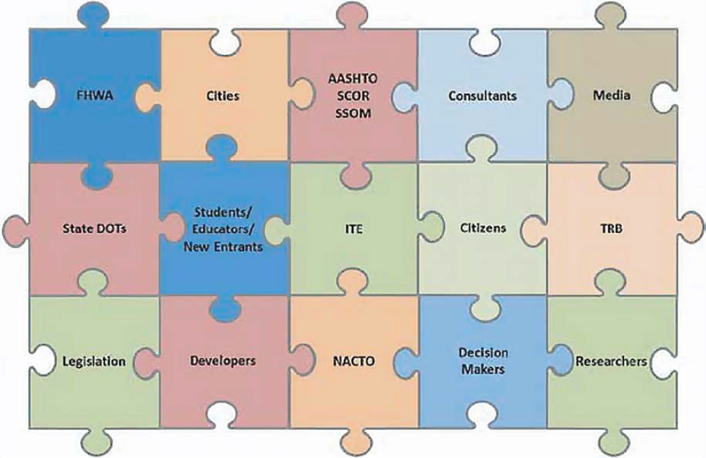
Another general resource under development is the TSSM. The TSSM is intended to serve as a guide for practitioners involved with all facets of operational traffic simulation and covers topics such as modeling resolutions, scenario development, and modeling processes, along with case studies and commentary on how to apply the guidance (List 2021). Many stakeholders have provided input into the TSSM’s development (see Figure 8). The TSSM has been transferred from FHWA to the TRB Standing Committee on Traffic Simulation for further development.
DOT Resources for Operational Traffic Simulation Models
This section presents the literature review of DOT resources for operational traffic simulation models.
Overview of Methodology for Review of DOT Resources for Operational Traffic Simulation Models
To inform the state of the practice, a literature review of published documentation regarding operational traffic simulation model development and calibration guidelines by individual states was conducted. Some materials were provided by the state DOTs through the survey that was conducted as part of this synthesis. Other materials were found through an Internet search engine by using phrases such as “state traffic analysis and simulation guidelines.”
Summary of Findings for Review of DOT Resources for Operational Traffic Simulation Models
Twenty-one state DOTs have one or more published guidelines or other documents detailing traffic simulation. A map of these state DOTs is shown in Figure 9. Ten of the published
ITE = Institute of Transportation Engineers
NACTO = National Association of City Transportation Officials
Source: FHWA 2017
Figure 8. TSSM structure.
documents contain traffic simulation guidance alongside the broader context of statewide traffic analysis guidelines; 11 are specific to operational traffic simulation (typically microsimulation). Nineteen of the publications provide specific resources associated with certain traffic simulation software, leaving only two that were software agnostic. Sixteen of the publications provide specific details for model coding and calibration, and 11 publications reference one or more model review checklists for use by state DOT reviewers or consultants.
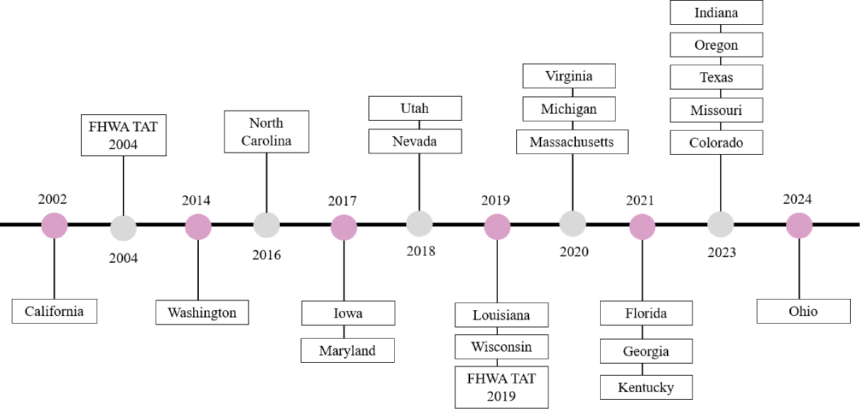
There is notable consistency and connection among the traffic simulation resources provided by state DOTs. Most DOT resources reference the TAT Volume III—both the 2004 and 2019 versions (Dowling et al. 2004; Wunderlich et al. 2019)—as well as at least one peer state DOT resource published previously. This means there is notable consistency among the recommended procedures for when to use operational traffic simulation, project scoping, model development, and model calibration among state publications. At the same time, each DOT resource offers a unique contribution through local data collected in its jurisdiction, specific operating procedures within the agency, strategies to enhance the accuracy and efficiency of producing traffic analyses, and detailed guidance on specific topics or model scenarios. A timeline for the development of guidance for operational traffic simulation models is shown in Figure 10.
The primary difference among state DOT resources is which simulation software the DOT requires, encourages, or promotes. Figure 11 shows the number of references to specific traffic simulation software in state DOT resources.
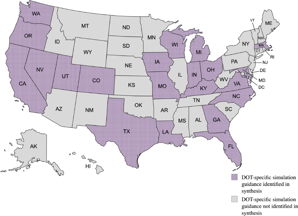
Figure 9. Map showing state DOTs with published guidelines or documents detailing traffic simulation.

Multiple states indicated that although they referenced a specific microsimulation software, the principles stated within their documentation apply to other similar software.
Similarities and differences in DOT guidance are discussed in greater detail in the following sections, organized by topic.
Details of DOT Resources for Operational Traffic Simulation Models
Most state DOT resources that cover operational traffic simulation models are built on the 2004 TAT. Each state-specific guideline was reviewed, and the six common elements described in this section were summarized from those guidelines.
Strategies for Selecting the Appropriate Traffic Analysis Tool
Traffic simulation modeling requires greater resources and effort and induces complexity (as compared to traditional analytical methods). For this reason, agencies have developed recommendations for situations in which traffic simulation should be used in place of deterministic methods (e.g., HCM, Synchro). Two-thirds (14 of 21) of the reviewed state DOT resources covered strategies for selecting the appropriate traffic analysis tool for a given project. In most cases, when referring to traffic simulation modeling, state DOTs are focused on microscopic models. These resources showed general agreement among states, highlighting that the benefits of traffic simulation modeling outweigh the costs under the following conditions: heavily saturated environments, unique traffic operations, and unique roadway geometries. A few excerpts from specific state DOT resources are provided in this subsection.
CDOT highlights the differences among traffic analysis tools—both modeling tools and deterministic tools—as shown in Figure 12.
The Florida DOT guidance conveys this same concept in a similar fashion, as shown in Figure 13. To supplement this figure, the guidance document states that “analysis of an isolated point or segment where influence from adjacent segments is marginal and congestion is not prevalent should always be performed by deterministic tools such as HCS or Synchro” (Florida DOT 2021).
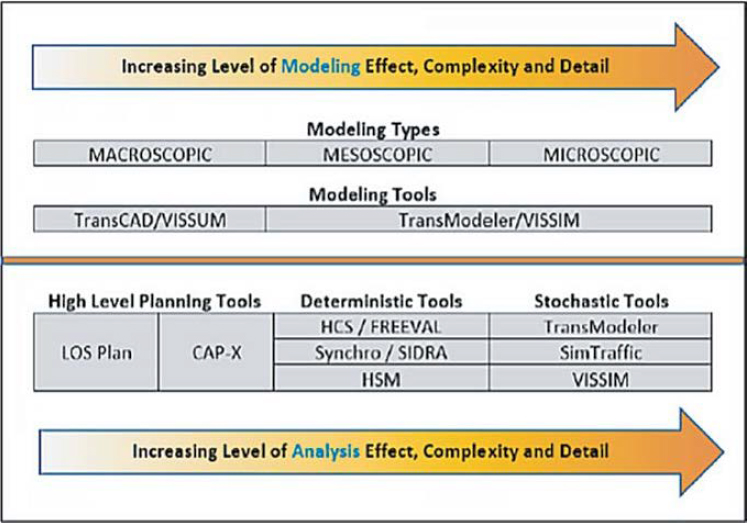
Figure 12. Traffic analysis tool degree of complexity for CDOT.

Figure 13. Traffic analysis tools for Florida DOT.
The Michigan DOT guidance outlines the following cases for which microsimulation software—in this case, PTV’s Vissim—is best applied:
Vissim is best applied for high-resolution operational analysis, where the nuances of the scenario to be tested fall outside the capabilities of other software packages. These may include:
- Complex signal timing or operations (such as transit signal priority or preemption strategies)
- Complex geometries
- Traffic flow and interaction through closely spaced intersections
- Managed-lane operations
- Ramp metering and active traffic management (ATM) strategies
- Roundabouts
- Curbside operations
- Connected vehicle/autonomous vehicle operations
- Interactions between nonmotorized and motorized modes of travel (Michigan DOT 2020).
The California DOT highlighted the following scenarios for which microsimulation should be used over other traffic analysis software:
- Conditions that violate one or more basic assumptions of independence required by HCM models (e.g., queues that spill back between intersections, city streets, and freeways)
- Conditions not covered well by available HCM models (e.g., roundabouts, signal pre-emption, unique lane configurations, truck climbing lanes, incident management options)
- Choosing Among Alternatives, None of Which Eliminate Congestion—analytical HCM techniques do not effectively distinguish between different levels of congestion (Level of Service “F”)
- Testing Options that Change Vehicle Characteristics and Driver Behavior (Dowling et al. 2002)
The Missouri DOT guidance categorizes analytical tools into four categories: sketch planning, travel demand models, analytical/deterministic, and microscopic simulation models (Missouri DOT 2023). Figure 14 provides a definition of each tool category, the pros and cons of leveraging tools within each category, and examples of software products leveraged by the DOT within each category.
The Kentucky Transportation Cabinet provides a table (shown in Figure 15) that highlights typical applications and relative level of effort for various traffic analysis tools, including simulation modeling tools. The traffic simulation software options introduced in the table include SimTraffic, Vissim, TransModeler, and Aimsun.
Project Scoping and Management
Several state DOT resources highlight standard practices for scoping and delivering traffic simulation modeling projects.
For example, the Utah DOT (UDOT) provides a diagram (shown in Figure 16) that demonstrates the typical organizational structure for traffic analysis projects—including the roles and responsibilities of the UDOT Traffic Management Division, the UDOT Region Traffic Engineers, and consultant traffic engineers (UDOT 2018). The UDOT Project Manager is responsible for directing the project and ensuring its completion. The Project Manager works directly with the consultant traffic engineers, who are often responsible for performing the traffic analysis. At the Project Manager’s discretion, involvement from the UDOT Traffic Management Division and UDOT Region Traffic Engineers may be requested.
The Oregon DOT developed a process diagram focused on the chapters of a standard traffic analysis report. This diagram (shown in Figure 17) demonstrates the interconnection between tasks associated with each chapter and specifies where tasks can be performed in parallel. This process broadly covers the traffic analyses that include traffic simulation models and those that do not.
Similarly, the Michigan DOT provides an eight-step series of milestones and deliverables that are used to guide microsimulation projects—in this case, using Vissim software—as shown in Figure 18. These milestones are divided into four stages: work prior to actual modeling, initial modeling, calibration, and model application (Michigan DOT 2020).
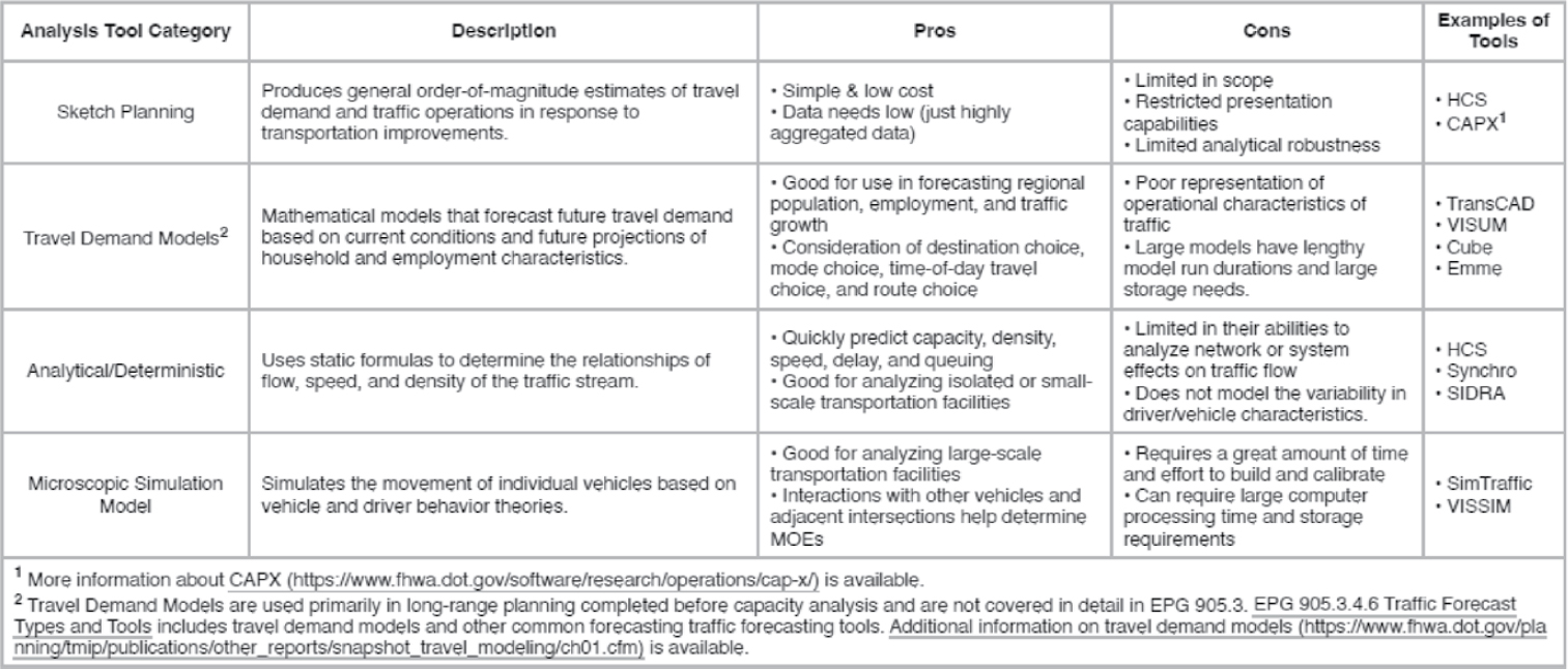
Figure 14. Traffic analysis tool categories for Missouri DOT.
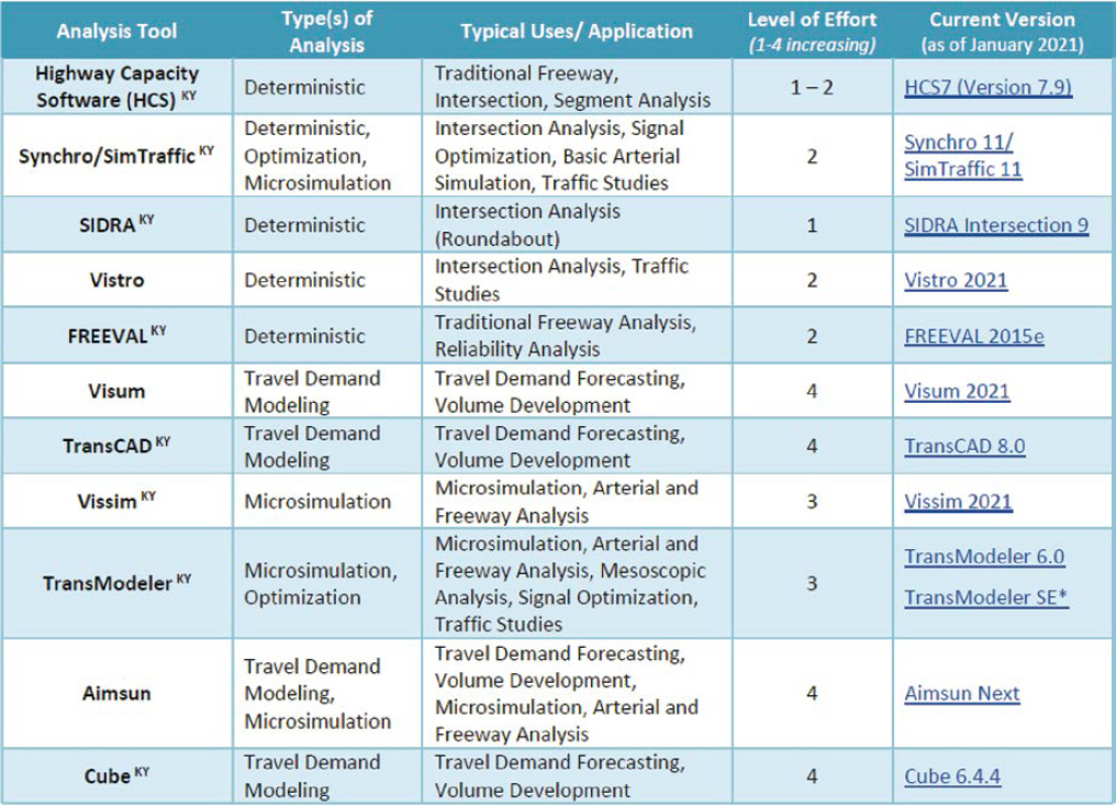
Figure 15. Traffic analysis tools for Kentucky Transportation Cabinet.
The Missouri DOT incorporates guidance from the TAT Volume 1 (Alexiadis et al. 2004), which includes seven considerations for traffic analysis projects that should be reviewed during the project scoping phase. These are geographic scope, facility type, travel mode, management strategy, traveler response, performance measures, and tool/cost-effectiveness (Missouri DOT 2023). Figure 19 highlights these considerations with additional detail.
Some DOTs include requirements for documenting methods and assumptions for traffic simulation modeling. For example, the Iowa DOT (2017) requires development of a methods and assumptions document for some projects. It stipulates that the document should be prepared in the early project stages and should address topics such as software tool selection, time periods, modeling extent, scenarios, data collection, targets for calibration, and MOEs. The Michigan DOT (2016) provides a template for a methods and assumptions document on its website.
Model Calibration Guidelines
The purpose of a simulation model is to investigate the impacts of the proposed improvement alternatives. Calibration refers to the adjustment of the model parameters to improve the model’s ability to reproduce observed traffic conditions. It is the required step during any traffic analysis in order to ensure that the model can reproduce local driver behavior and traffic performance characteristics; calibration should be done prior to evaluating alternatives. Most traffic simulation models are designed to be flexible enough that an analyst can correctly calibrate the network to match the location conditions at a reasonably accurate level. However, the default values will rarely give accurate results for a specific area. Therefore, calibration is necessary in order to adjust the Vissim model parameters to replicate the traffic characteristics of the study area.
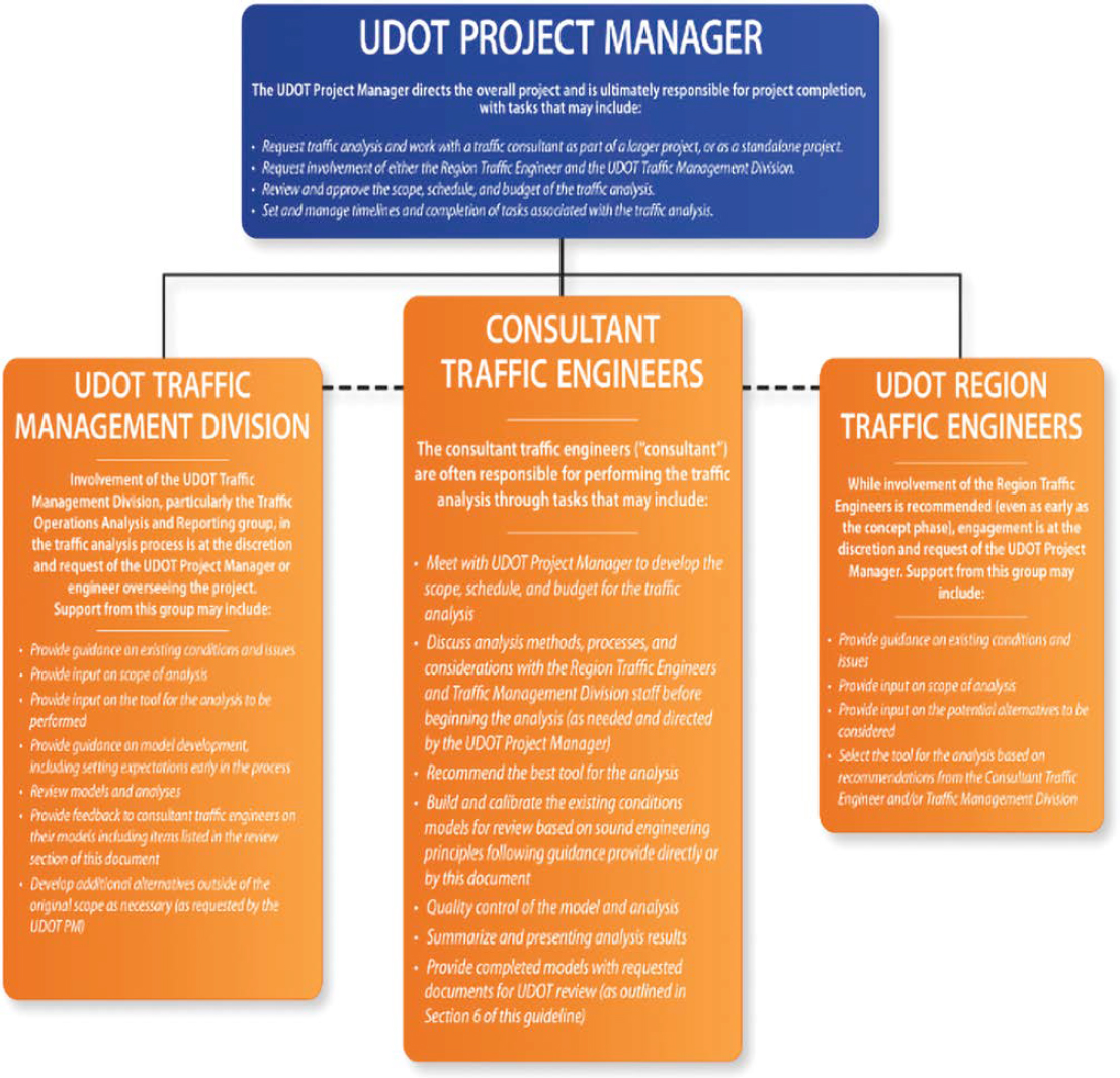
Figure 16. Team organizational structure and overview of roles and responsibilities for UDOT.

Figure 17. Process of traffic analysis for Oregon DOT.
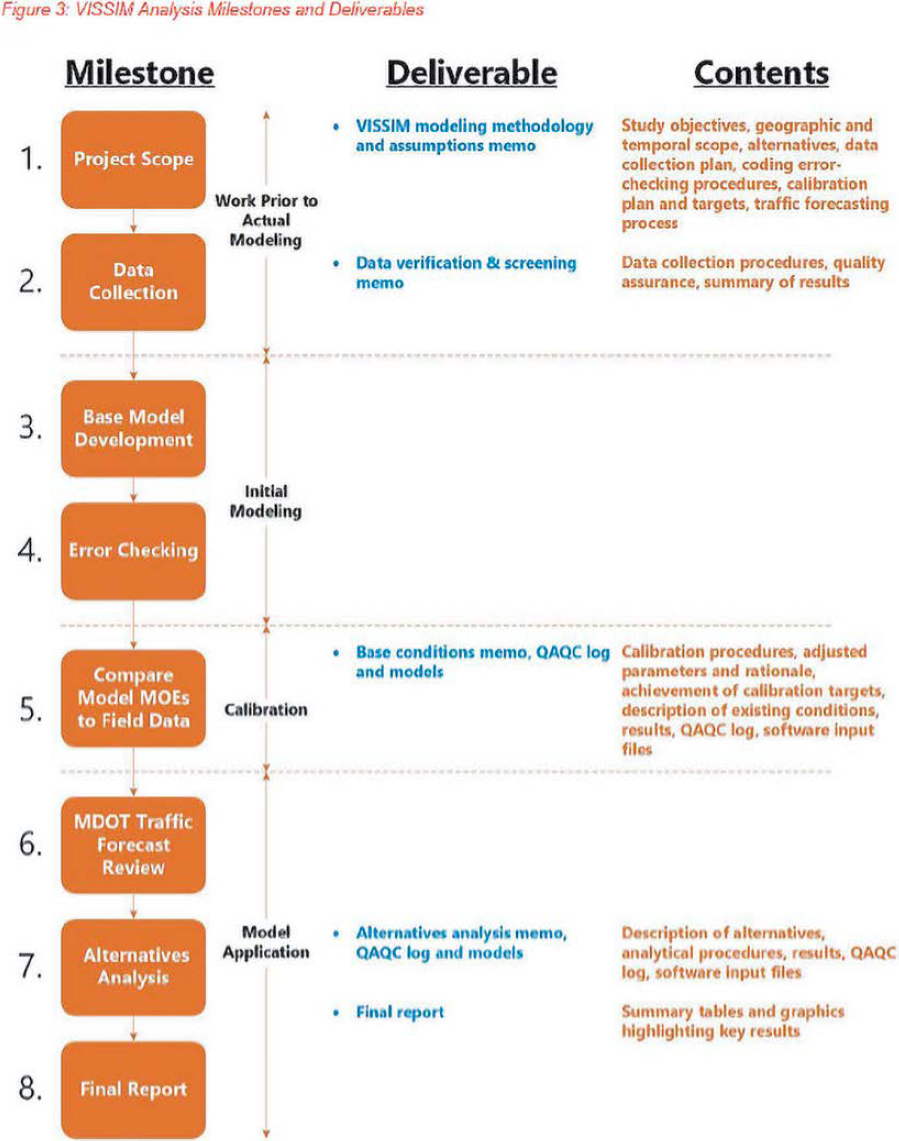
Figure 18. Vissim analysis milestones and deliverables for Michigan DOT.

Figure 19. Considerations for determining a project’s analytical context.
Calibration Targets
Typically, state DOTs use variations of the 2004 TAT calibration targets (Dowling et al. 2004), with slight modifications that frequently reference peer states. Simulation model calibration is performed during model development in existing conditions for the purpose of comparing the model outputs with real system performance. Nearly all state DOT resources use the following measures of simulation model calibration:
- Throughput on individual vehicle links. This is measured within a certain percentage or count of the actual vehicle numbers on every link. For example, 85% of all links within the network are required to fall within 15% of throughput when volume is between 700 and 2,700 vehicles per hour, within 100 vehicles when volume is less than 700 vehicles per hour, or within 400 vehicles per hour when volume is greater than 2,700 vehicles per hour (Dowling et al. 2002). There are slight variations among DOTs on the exact volume, error threshold, and link requirement used; however, all DOTs use some form of link-level volume comparison. For example, the Virginia DOT (VDOT) requires 85% of the network links, in addition to 100% of the “critical” links (as determined by the district traffic engineer), to meet its specific volume criteria (VDOT 2020a).
- Overall vehicle throughput. This is a comparison of the overall percentage difference in volume measured in the model and from actual vehicle counts on each input link into the
- network. For example, a requirement may be that the percentage difference in total network throughput should be within 5% (Florida DOT 2021; Dowling et al. 2002).
- GEH statistic of individual and total link throughputs. The GEH statistic is used for comparing two sets of traffic volumes and is similar to a chi-squared test. In this case, the two sets of traffic volumes represent the simulated model volumes and the actual vehicle counts. For example, a requirement may be that 85% of links should have a GEH statistic of less than 5, and the combination of all input links should have a GEH statistic of less than 4 (Florida DOT 2021; Dowling et al. 2002).
- Travel times on designated routes. This is a comparison of the percentage or absolute difference between travel times collected in the field and those collected through the simulated model. For example, a requirement may be that 85% of travel time routes should be within a 15% difference or one minute, whichever is higher (Dowling et al. 2002). VDOT specifies that 85% of travel time routes must be within 30% for arterials and 20% for freeways (VDOT 2020a). Similar to the link throughput calibration, all state DOT resources reference a similar travel time calibration criterion as provided in the example. Since the length and quantity of travel time routes can make a big difference in determining the calibration accuracy, some state DOTs also specify specific routes as “critical” and that these must meet the criteria (VDOT 2020a). Other states specify the time duration that should be measured. For example, CDOT requires that travel times be measured on 15-minute intervals for calibration (CDOT 2023).
- Queue lengths, bottlenecks, and individual link speeds. The greatest differences in calibration thresholds among states are related to queue lengths, bottlenecks, and speeds. A few state DOTs require quantitative comparison of these measures. For example, they may require that simulated and observed queue lengths must be within 20% and simulated link speeds must be within 10 miles per hour (mph) of field-measured speeds (Florida DOT 2021). Other DOTs (those of Virginia, Colorado, and California) require visual audits or qualitative comparison of expected congestion patterns from the field, with simulated congestion patterns from the model at key locations (VDOT 2020a; CDOT 2023; Dowling et al. 2002).
In its 2019 manual, the Wisconsin DOT made significant updates to its calibration requirements, which formerly were similar to the 2004 TAT requirements and those of most other state DOTs (Wisconsin DOT 2005). The Wisconsin DOT introduced a two-tiered approach to model calibration; the first tier checks global characteristics of the model, and the second tier checks local characteristics of the model. If a model passes all required checks from the first tier, it is not required to move to the second tier. In most cases, the calibration checks use the Root Mean Squared Percentage Error and Root Normalized Squared Error to compare field data with simulation outputs for volume, speed, travel time, queue lengths, and lane use (Wisconsin DOT 2019).
Acceptable Calibration Values
In addition to calibration thresholds, state DOTs typically provide or reference acceptable parameters and value ranges for model calibration. The most commonly adjusted calibration parameters include those used to define driving behavior, specifically those controlling car-following models (i.e., determining each vehicle’s longitudinal motion) and lane-changing models (i.e., determining each vehicle’s lateral motion).
The Kentucky Transportation Cabinet provides an in-depth guide to parameter selection for both Vissim and TransModeler, derived by local data. The snapshot of this tool, shown in Figure 20, illustrates one sheet (within the overall spreadsheet) that is focused on the recommended parameter range for calibration parameter “cc1: time headway” commonly used in the Wiedemann 1999 car-following model inherent within Vissim. As shown in Figure 20, not only is the recommended range provided (i.e., 0.7–1.6 seconds), but the distribution supporting those values is also provided (Kentucky Transportation Cabinet 2021).
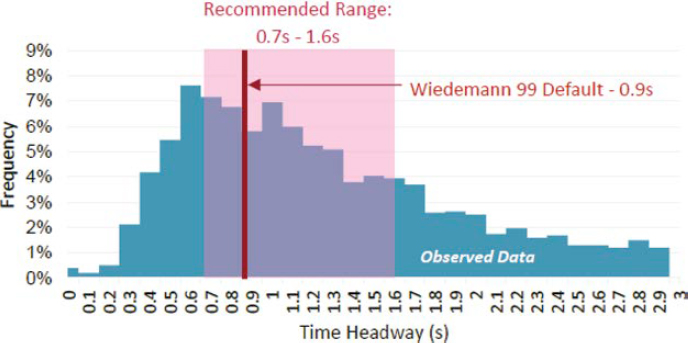
Figure 20. Microsimulation parameter quick reference spreadsheet for Kentucky Transportation Cabinet.
Calibration Procedures
Model calibration is an iterative process that is difficult to detail in a step-by-step manner, as each model has distinct steps that are required to achieve calibration. Approximately half of DOTs offer recommended calibration strategies similar to those of the California DOT, which suggests the following process:
- Check for and eliminate all obvious coding errors.
- Calibrate the capacity related adjustment factors.
- Calibrate the demand estimation parameters.
- Review the overall realism of model results—queues and travel times (Dowling et al. 2002).
As shown in Figure 21, VDOT offers a calibration flowchart that provides pre-calibration steps, freeway calibration steps, and arterial network calibration steps. This guide recommends specific parameters associated with Vissim microsimulation software to adjust iteratively in tandem and in isolation of other parameters. Different steps are provided for freeways and arterial corridors due to the unique interactions between vehicles in these environments and the different driving behavior models typically used in each environment. The Vissim vendor, PTV, recommends using Wiedemann 99 for freeway traffic with no merging areas and Wiedemann 74 for urban traffic and merging areas in Vissim models (PTV Group 2019). Each of these car-following models has different parameters and differences in traffic control between environments (e.g., merge/diverge/weaves at ramp junctions versus traffic signals and stop signs). The VDOT Vissim User Guide provides additional detail to modelers regarding each of these steps (VDOT 2020b).
2019 FHWA Calibration Guidelines
Review Checklists
Eleven of the 21 DOT resources reviewed include traffic simulation model review checklists. These checklists vary in length, specificity, and content; however, most include the following core information:
- Network coding (e.g., links, connectors)
- Control devices (e.g., stop signs, signal heads, detectors, traffic signal controllers and their timing)
- Base data (desired speed distributions, vehicle composition)
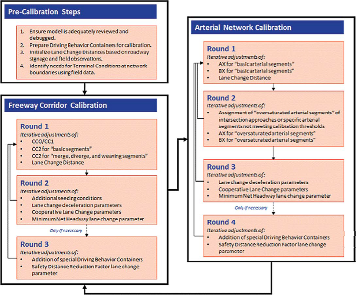
Figure 21. Flowchart of calibration steps for VDOT.
- Driving behavior (car-following, lane-change, acceleration parameters)
- Vehicle inputs and routing (link-level volumes throughout the corridor)
- Conflict prioritization at intersections and other junctions
- Multimodal demand and coding (e.g., pedestrian, bicycle, transit)
- Performance measure outputs (e.g., volume, travel time, queue length, link speeds)
- Core simulation parameters (simulation seeds, evaluation criteria)
- Model errors (review of error log and visual audits of stuck/stalled vehicles or otherwise unrealistic behavior)
- Calibration/validation thresholds and parameters
- Result consistency with related traffic models
- Documentation
Table 2 provides a summary of DOT resources that contain checklists, including their URLs.
Table 2. Summary table of DOT resources with checklists.
The Wisconsin DOT developed a policy for model review to improve consistency across the state. In addition to creating a detailed checklist, the agency developed a process to define the level of review required for a given project. The four levels of review are (1) project team level review, (2) region level review, (3) independent consultant level review, and (4) statewide bureaus level review with FHWA oversight. To determine which level of review is required for a given project, the DOT created a scoring system based on project type, geometric conditions, and traffic operational conditions. This scoring rubric is illustrated in Figure 22. The complexity of each facet of the model development process is determined, and the sum of scores is used to determine the level of necessary peer review. For example, a complexity score of 0–3 only requires project team level review, whereas a score of greater than 11 requires statewide bureaus level review with FHWA oversight (Wisconsin DOT 2019).
Training Materials
A few state DOTs have developed and published training materials related to traffic simulation models. For example, as part of the California DOT manual, sections were written with “laboratory sessions” that walk a reader through an example of completing a related task. These sessions include microsimulation model calibration; assessment of microsimulation results; and scoping, budgeting, and scheduling a microsimulation project (Dowling et al. 2002).
The Georgia DOT developed a series of eight educational modules to aid in the development of Vissim microsimulation model skills within the agency. The first four modules introduce arterial and freeway corridor model development, and the final four modules cover broader modeling topics such as working with model outputs, model calibration, and model review (Hunter 2021).
Research Studies on Operational Traffic Simulation Models
This section presents the literature review of research studies on operational traffic simulation models, including applications, modeling resolution, modeling processes, software tools, and visualization.
Applications of Operational Traffic Simulation Models
Operational traffic simulation models have been used for various applications such as CAVs, design, operations, environmental impacts, and multimodal contexts. Examples of these applications in the literature are presented in the following sections. Additional details, including other studies, can be found in Appendix D.
Application of Operational Traffic Simulation Models to Connected and Automated Vehicles (CAVs)
Several research studies have investigated various aspects of modeling CAVs using simulation. Beza et al. (2022) explored the calibration of the Vissim microscopic traffic simulation software for simulating different types of automated vehicles (AVs). Their findings revealed that certain parameters for AVs, such as standstill distance and headway time, can be expected to have lower values than those of conventional vehicles, while parameters such as standstill acceleration and looking distances may have higher values than those of conventional vehicles. Kim et al. (2021) evaluated the impact of CAVs on Virginia freeway corridors and found that AVs and CAVs can significantly increase road capacity, with CAVs showing potential for lowering traffic congestion as demand grows. Manjunatha et al. (2022) assessed the capability
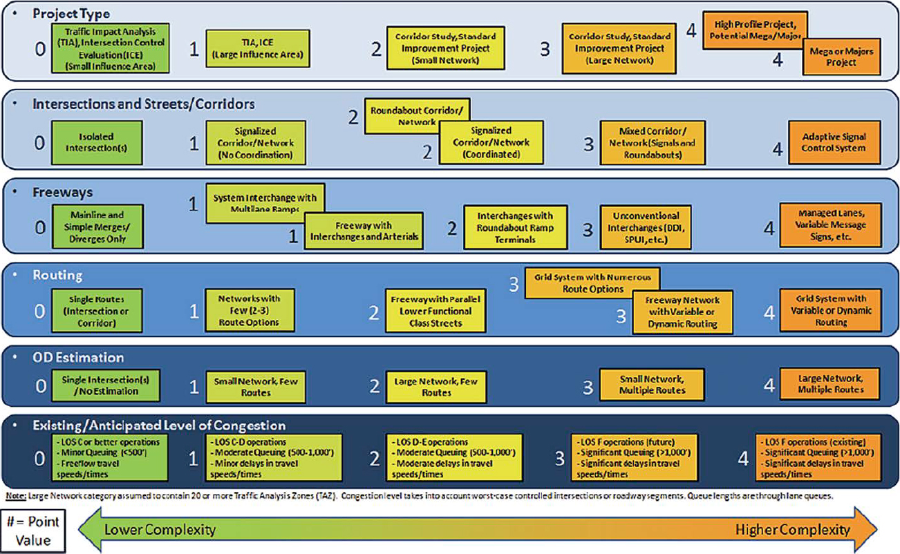
Figure 22. Traffic model complexity scoring diagram for Wisconsin DOT.
of microsimulation to model CAVs and introduced a comprehensive CAV model extension. They noted some of the limitations of microsimulation for modeling CAVs, such as the complex behavior of vehicles and modeling connectivity. Sha et al. (2023) developed a novel calibration framework for traffic simulation models, focusing on safety and operational measures for connected vehicle (CV) applications.
Application of Operational Traffic Simulation Models to Design
Example applications of operational traffic simulation models to design include passing sight distance (PSD), freeway weaving sections, and modifications in street design. Haq et al. (2022) used microsimulation to validate results of an existing kinematics model for PSD. Lee et al. (2023) investigated the effects of weaving length under various traffic conditions at freeway weaving sections using microsimulation. Liu et al. (2021) applied microsimulation to assess the impacts of conversion from one-way to two-way streets in San Jose, California, incorporating the effects of different travel demand levels and movements of vehicles, pedestrians, and bicycles.
Application of Operational Traffic Simulation Models to Assessment of Environmental Impacts
Simulation modeling has been used to explore environmental impacts such as noise, emissions, and fuel consumption. Baclet et al. (2023) developed methodology for real-time dynamic noise mapping using microscopic traffic simulation and applied it to a city in Estonia. Song et al. (2020) investigated the performance of two traffic simulation packages in capturing nontraffic measures such as fuel consumption, emissions, and safety. Despite calibration based on traffic indicators, the researchers found that the simulation accuracy in predicting these measures was not sufficient. Guin et al. (2023) tested emission differences between a Restricted Crossing U-Turn intersection and a traditional intersection through simulation. Results showed an overall reduction in intersection emissions in scenarios with a sufficiently large mainline volume to side street ratio.
Application of Operational Traffic Simulation Models to Multimodal Contexts
Microsimulation has also been used for evaluations related to other travel modes, including pedestrian, bicycle, and transit. For example, Gavric et al. (2023) introduced two novel pedestrian timing treatments and evaluated them using microsimulation. Results indicated that the novel treatments led to better performance than conventional treatments for pedestrian timing. Kodupuganti and Pulugurtha (2023) assessed how light rail transit and nonmotorized modes of travel affect vehicle delays at intersections by using microsimulation on a corridor in Charlotte, North Carolina. Results indicated that the light rail transit improved main street traffic performance, whereas nonmotorized traffic increased delays. Lemcke et al. (2021) explored the use of Vissim and the Surrogate Safety Assessment Model to calibrate microscopic simulations to field-observed bicycle–vehicle conflicts. The results indicated that default driving behavior parameters in Vissim underestimate such conflicts as compared to field data, demonstrating a need for adjustments and further research to understand the effects of microsimulation user behavior parameters on reported conflicts. Sultan et al. (2023) assessed the operational performance of transit signal priority using microsimulation.
Application of Operational Traffic Simulation Models to Operations
Operational traffic simulation models have been implemented in various applications for operations, such as for rail crossings, weather effects, rideshare, and Transportation Systems Management and Operations (TSMO) strategies. Creasey and Choi (2023) conducted two case
studies using microsimulation and created a framework to guide practitioners and decision-makers in performing traffic operations analyses for at-grade rail crossings. An example graph of observed and simulated duration of traffic interruption time is shown in Figure 23. Das and Ahmed (2022) outlined a method to refine microsimulation models with weather-specific lane-change parameters and applied the method to segments of I-80 in Wyoming. The updated models revealed that bad weather leads to more traffic conflicts, reduced speeds, and higher travel times and delays. Wang et al. (2022) developed a detailed curbside driving behavior model to address changes in travel patterns due to the increased prevalence of ridesharing. Williams et al. (2011) delivered a calibrated dynamic traffic assignment (DTA) model for the Triangle region in North Carolina, providing assessment capabilities for operational strategies such as including high-occupancy vehicle or high-occupancy toll lanes, congestion pricing, ramp metering, signal coordination, incident management, and traveler information.
Other Applications of Operational Traffic Simulation Models
Other applications of operational traffic simulation models presented in the literature include evacuation modeling and evaluating defense installations. Chang and Edara (2018) implemented a reservation-based intersection control algorithm for hurricane evacuation in a CAV environment using a Virginia road network simulation and found that the algorithm led to increased speeds and reduced delay. Naser and Birst (2010) created a hybrid evacuation model for urban areas by combining traffic simulation with a traditional transportation planning model and modeled multiple scenarios for emergency evacuation in the Fargo-Moorhead metropolitan area in North Dakota. The evacuation modeling methodology is shown in Figure 24. Carter and Rilett (2023) introduced a microsimulation-based methodology for analyzing the design and operations of entry control facilities at Department of Defense installations and demonstrated the methodology through an evaluation of geometric and operational alternatives for an entry control facility in Georgia.
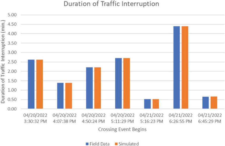
Figure 23. Duration of traffic interruption due to train crossing in Cotulla, Texas.

Figure 24. Hybrid evacuation modeling methodology for Fargo-Moorhead metropolitan area.
Macroscopic Simulation Modeling
Macroscopic simulation modeling has been used for signal optimization and large-scale evacuation planning. Chen and Chang (2014) a developed a generalized signal optimization model for arterials that were handling multiclass traffic flows, utilizing a macroscopic simulation concept to capture complex interactions among different vehicle types. The model outperformed other software, especially in congested and multiclass traffic scenarios. Lieberman and Xin (2012) introduced a new macroscopic traffic flow model that was used in the large-scale evacuation planning software DYNEV II. The model is designed for generalized networks, accommodating longer simulation time steps (of one minute or more) to reduce computational cost and interfacing with a DTA model.
Mesoscopic Simulation Modeling
Research on mesoscopic simulation modeling has focused on areas such as calibration and validation and heterogeneous traffic characteristics. Zhao and Appiah (2021) presented a new calibration and validation procedure for mesoscopic models and successfully tested the procedure on a real-world highway network with sufficient calibration results. Pi et al. (2019) developed and implemented a large-scale mesoscopic DTA model that incorporated separate demand and flow dynamics for cars and trucks and illustrated the use of the model through a case study. Zhu et al. (2018) introduced an integrated approach that combines DTA with a positive agent-based microsimulation travel behavior model to evaluate the cumulative impact of land development on transportation infrastructure and demonstrated the approach using a congested corridor in Maryland.
Multiresolution Modeling (MRM)
Studies on MRM have developed systems and investigated applications such as dynamic reversible lane systems and work zones. Li et al. (2015) developed a multiresolution traffic simulation system for comprehensive metropolitan area modeling through the integration of mesoscopic and microscopic simulators. The approach, which was demonstrated with a case study, begins with the microscopic simulation network and then moves to the mesoscopic network. Nava et al. (2012) deployed an MRM methodology, including simulation-based DTA, using a mesoscopic model and a more detailed analysis of MOEs using a microscopic model of a subarea. The study focused on identifying traffic-related issues and advantages in implementing and operating dynamic lane closure and reversible lane strategies on the I-70 corridor near Denver, Colorado. Shelton et al. (2012) used MRM techniques to calculate road user costs and analyze the system-wide effects of traffic diversion due to work zones. Their approach incorporated a sub-area converted to a microscopic level to obtain MOEs in order to capture driver behavior due to delays from route changes.
Processes for Simulation Modeling
The existing literature on processes for simulation modeling covers topics such as calibration tools and processes and car-following models. Xue et al. (2019) explored the effectiveness of using unmanned aerial vehicles to validate traffic simulation model outputs for an intersection in Auburn, Alabama. The traffic simulation models were calibrated and compared with high-resolution video and photographic data collected by unmanned aerial vehicles. Yang and Zhou (2023) developed calibration methods for Vissim simulation models of direct left turn movements and right turn followed by U-turn movements at unsignalized intersections on rural divided highways by using Naturalistic Driving Study data.
Research studies have investigated the use of automation or algorithms to enhance the calibration process. Tang et al. (2023) proposed an automated method for sensitivity analysis of microscopic traffic simulation parameters using the Component Object Model interface technology provided by Vissim simulation software to simulate 20 key parameters. The results indicated the importance of parameters such as headway, following state, average expected distance, and following variable in affecting the calibration index for toll stations. Shahrokhi Shahraki et al. (2018) proposed a soft-computing-based methodology, incorporating a combination of artificial neural networks and genetic algorithms, to significantly reduce the computation time for calibrating vehicular microscopic simulation models.
Other research has focused on car-following models. James et al. (2019) used trajectory-level driving data to refine car-following models. They evaluated eight methods to aggregate diverse driving behaviors into representative parameter sets. Results showed that methods that averaged behavior while preserving parameter correlations were the most effective. Simpler approaches, such as using mean or median values of parameters, also proved practical and surpassed default model parameters in performance. Kaths et al. (2021) investigated the adaptation of the psycho-physical Wiedemann 99 car-following model—commonly used in microscopic traffic simulations—for bicycle traffic, based on microscopic trajectory data from a bicycle simulator study. The results demonstrated improved realism in simulating bicycle traffic with the calibrated model, although meeting the observed variation in average queue dissipation times did not occur with the tested parameter sets.
Simulation Software
Researchers have investigated different software packages used for operational traffic simulation models. Pell et al. (2017) compared 17 simulation software packages through a literature review, survey, and interviews with practitioners. They found that the programs were able to model current and traffic conditions, but no single system provided all functionalities. They also identified a need for online simulation software applications targeted toward heterogeneous transportation networks in mixed-use areas. Ullah et al. (2021) analyzed 29 software packages and found that the choice of software depends on factors such as local traffic conditions, driver behavior, and type of road infrastructure. Jones et al. (2004) reviewed three simulation packages for analyzing transportation system alternatives and found that each package has its own strengths and may be suitable for specific applications. Shaaban and Kim (2015) compared the performance of SimTraffic and Vissim in modeling dual lane and triple lane roundabouts and found that the two tools generally did not show statistically significant differences in results.
Visualization of Simulation Results
A limited number of studies have discussed the use of operational traffic simulation models for visualization. For example, Wilson Simao et al. (2023) migrated Vissim data into a 3D digital model of a corridor and integrated the model into an augmented reality application to help the public to visualize corridor improvements. Xu et al. (2022) developed a web-based application to facilitate archiving, sharing, and visualization of large-scale traffic simulation outputs to help address the challenges of managing, disseminating, and visualizing traffic simulation results.


