Reference Manual on Scientific Evidence: Fourth Edition (2025)
Chapter: Reference Guide on Epidemiology
Reference Guide on Epidemiology
STEVE C. GOLD, MICHAEL D. GREEN, JONATHAN CHEVRIER, AND BRENDA ESKENAZI
Steve C. Gold, J.D., is Professor of Law and Judge Raymond J. Dearie Scholar, Rutgers Law School, Rutgers University–Newark, Rutgers, The State University of New Jersey.
Michael D. Green, J.D., is Visiting Professor, Washington University in St. Louis School of Law.
Jonathan Chevrier, Ph.D., is Associate Professor of Epidemiology, Department of Epidemiology, Biostatistics and Occupational Health, School of Population and Global Health, Faculty of Medicine and Health Sciences, McGill University.
Brenda Eskenazi, Ph.D., is Professor Emeritus of Maternal and Child Health and Epidemiology, School of Public Health, University of California at Berkeley.
CONTENTS
The Different Kinds of Epidemiologic Studies
Experimental and Observational Studies of Suspected Toxic Agents
Types of Observational Study Design
Genetic and Molecular Epidemiologic Studies
Epidemiologic and Toxicologic Studies
Interpreting the Results of an Epidemiologic Study
Internal and External Validity
Sources of Error in Epidemiologic Studies
Information bias due to misclassification
Techniques to identify confounding factors
Techniques to prevent or limit confounding
Techniques to control for confounding factors
Biases That Affect a Body of Epidemiologic Evidence
Consideration of Alternative Explanations
Specificity of the Association
Consistency with Other Relevant Knowledge
Methods for Synthesizing or Combining the Results of Multiple Studies
Qualifications of Experts in Epidemiology
FIGURES
2. Design of a case-control study
3. Risks in exposed and unexposed groups
5. 90% and 95% confidence intervals for a hypothetical study with a relative risk of 1.5
6. Directed acyclic graph (DAG) for a hypothetical study of glyphosate and non-Hodgkin lymphoma
7. Directed acyclic graph for a hypothetical study of air pollution and heart disease
10. Linear threshold dose response
11. Supra-linear dose response
13. Non-monotonic dose response
TABLES
1. Cross Tabulation of Exposure by Disease Status
2. Cross Tabulation of Cases and Controls by Exposure Status
Introduction
Epidemiology is the field of public health and medicine that studies the occurrence, distribution, and determinants of health and disease in human populations. The purpose of epidemiology is to better understand disease causation and to prevent disease in groups of individuals.1 Epidemiology assumes that disease is not distributed randomly in a group of individuals and that identifiable subgroups, including those exposed to certain agents, are at increased risk of contracting particular diseases.2
Judges and juries increasingly are presented with epidemiologic evidence as the basis of an expert’s opinion on causation.3 In the courtroom, epidemiologic research findings are offered to establish or dispute whether exposure to an agent4 caused a harmful effect or disease.5 Since Daubert v. Merrell Dow
1. More generally, epidemiologists study and seek to improve health outcomes in populations; this may go beyond the study of “diseases.” For example, an epidemiologist might be interested in suspected causes of osteoarthritis of the knee (a health outcome that is a disease) and also in interventions thought to improve osteoarthritic knees’ range of motion (a health outcome that is not a disease). In this reference guide, we generally refer to the dependent variable being assessed in an epidemiologic study as a health outcome. In certain contexts, however, we use the term disease, because a plaintiff’s disease is the type of outcome most often at issue in cases in which epidemiology serves as evidence of causation. In any case, in the legal context, references to health outcomes or diseases should be understood, unless stated otherwise, as constituting adverse changes that are legally cognizable. In addition, in this reference guide we generally discuss outcomes as if they are discrete variables that either are present or absent (such as cancer), even though many health outcomes are continuous variables (such as blood pressure or body mass index).
2. Epidemiologists also conduct studies of beneficial agents that reduce disease risk or that prevent or cure disease or otherwise improve health outcomes.
3. Epidemiologic studies have been well received by courts deciding cases involving toxic substances. See, e.g., Norris v. Baxter Healthcare Corp., 397 F.3d 878, 882 (10th Cir. 2005) (“[E]pidemiology is the best evidence of general causation in a toxic tort case.”); Newman ex rel. Newman v. McNeil Consumer Healthcare, No. 10 C 1541, 2013 WL 9936293, at *10 (N.D. Ill. Mar. 29, 2013) (“Epidemiological studies are important . . . [and provide] ‘the primary, generally accepted methodology for demonstrating a causal relation between a chemical and a set of symptoms or a disease.’” (quoting Conde v. Velsicol Chem. Corp., 804 F. Supp. 972, 1025–26 (S.D. Ohio 1992), aff’d, 24 F.3d 809 (6th Cir. 1994))). Well-conducted studies are uniformly admitted. 3 Modern Scientific Evidence: The Law and Science of Expert Testimony § 23.1, at 321 (David L. Faigman et al. eds., 2021–2022) [hereinafter Modern Scientific Evidence].
4. We use the term agent to refer to any substance external to the human body that potentially causes disease or other health effects. Drugs, medical devices, chemicals, radiation, vaccines, pathogens (e.g., viruses or bacteria), and minerals (e.g., asbestos) are all agents whose toxicity an epidemiologist might explore. A single agent or a number of independent agents may cause disease, or the combined presence of two or more agents may be necessary for the development of the disease. Epidemiologists also conduct studies of individual characteristics that might pose risks, such as blood pressure and diet, but those studies are rarely of interest in judicial proceedings except as possible alternative causes to an alleged tortious cause. Epidemiologists also may conduct studies of drugs and other pharmaceutical products to assess their efficacy and safety in clinical trials.
5. E.g., In re Testosterone Replacement Therapy Prods. Liab. Litig. Coordinated Pretrial Proc., No. 14 C 1748, 2017 WL 1833173 (N.D. Ill. May 8, 2017) (assessing whether plaintiffs’ arterial
Pharmaceuticals,6 the predominant use of epidemiologic studies is in connection with motions to exclude the testimony of expert witnesses. Courts deciding such motions routinely address epidemiologic studies and whether they are sufficient to support an expert’s causation testimony.7
Epidemiology aims to develop evidence to identify agents that are associated with an increased risk of disease in groups of individuals, quantify the amount of excess disease that is associated with an agent, and attempt to provide a profile of the type of individual who is more likely to contract a disease after being exposed to an agent. Epidemiology focuses on the question of general causation (i.e., is the agent capable of causing disease?) rather than that of specific causation (i.e., did it cause disease in a particular individual?).8 For example, in the 1950s, Doll and Hill and others published articles about the increased risk of lung cancer in cigarette smokers. Doll and Hill’s studies showed that smokers
cardiovascular injuries or venous thromboembolisms were caused by prescription testosterone-replacement-therapy drugs); In re Mirena IUD Prods. Liab. Litig., 169 F. Supp. 3d 396 (S.D.N.Y. 2016) (assessing whether uterine perforation was caused by intrauterine devices); In re Lipitor (Atorvastatin Calcium) Mktg., Sales Pracs. & Prods. Liab. Litig., 174 F. Supp. 3d 911 (D.S.C. 2016) (assessing whether Lipitor caused the development of type 2 diabetes); In re E.I. du Pont de Nemours & Co. C-8 Pers. Inj. Litig., No. 2:13-MD-2433, 2015 WL 4092866 (S.D. Ohio July 6, 2015) (assessing whether water sources contaminated with ammonium perfluorooctanoate (C-8, or PFOA) caused residents to develop certain diseases, including testicular cancer and preeclampsia).
6. 509 U.S. 579 (1993).
7. See Michael D. Green & Joseph Sanders, Admissibility Versus Sufficiency: Controlling the Quality of Expert Witness Testimony, 50 Wake Forest L. Rev. 1057 (2015). Often the expert witness in a case in which a study bears on causation is not the investigator who conducted the study. See, e.g., DeLuca v. Merrell Dow Pharms., Inc., 911 F.2d 941, 953 (3d Cir. 1990) (holding a pediatric pharmacologist expert’s credentials sufficient pursuant to Fed. R. Evid. 702 to interpret epidemiologic studies and render an opinion based thereon); In re Deepwater Horizon Belo Cases, No. 3:19CV963-MCR-HTC, 2022 WL 17721595, at *13 (N.D. Fla. Dec. 15, 2022) (stating that non-practicing physician who worked in public health and biomedical research was qualified to testify about general causation); Donner v. Alcoa Inc., No. 10-CV-00908-DW, 2014 WL 12600281, at *5 (W.D. Mo. Dec. 19, 2014) (holding admissible a pathologist’s opinion about general and specific causation regarding exposure to aluminum dust and pulmonary fibrosis); Watson v. Dillon Cos., Inc., 797 F. Supp. 2d 1138, 1162 (D. Colo. 2011) (holding medical doctors’ opinions about general and specific causation regarding inhalation of butter flavoring ingredients in microwave popcorn and a rare lung condition were admissible); Sugarman v. Liles, 190 A.3d 344, 345–68 (Md. 2018) (holding admissible a physician’s testimony about general and specific causation regarding lead paint and cognitive injuries).
8. The distinction between general causation and specific causation is widely recognized in court opinions. See, e.g., Norris v. Baxter Healthcare Corp., 397 F.3d 878, 881 (10th Cir. 2005) (“Plaintiff[s] must first demonstrate general causation because without general causation, there can be no specific causation.”); Harrison v. BP Expl. & Prod. Inc., No. CV 17-4346, 2022 WL 2390733, at *4 (E.D. La. July 1, 2022) (“Once a plaintiff’s diagnoses have been confirmed, the plaintiff has the burden of establishing general causation and specific causation.”); Rhyne v. United States Steel Corp., 474 F. Supp. 3d 733, 743 (W.D.N.C. 2020) (“Plaintiffs must prove both general causation and specific causation.”). For a discussion of specific causation, see the section titled “Specific Causation” below.
who smoked 10 to 20 cigarettes a day had a lung-cancer mortality rate that was about 10 times higher than that of nonsmokers.9 These studies identified an association between smoking cigarettes and death from lung cancer that contributed to the determination that smoking causes lung cancer.
However, it should be emphasized that an association is not equivalent to causation.10 An association is the relationship between two events (e.g., exposure to a chemical agent and development of disease) that occur more frequently together than one would expect by chance. An association identified in an epidemiologic study may or may not be causal.11
Assessing whether an association is causal requires an understanding of the strengths and weaknesses of the study’s design and implementation, as well as a judgment about how the study findings fit with other similar studies and
9. Richard Doll & A. Bradford Hill, Lung Cancer and Other Causes of Death in Relation to Smoking: A Second Report on the Mortality of British Doctors, 2 Brit. Med. J. 1071 (1956), https://doi.org/10.1136/bmj.2.5001.1071.
10. In In re Lipitor (Atorvastatin Calcium) Mktg., Sales Pracs. & Prod. Liab. Litig., 227 F. Supp. 3d 452 (D.S.C. 2017), aff’d sub nom. In re Lipitor (Atorvastatin Calcium) Mktg., Sales Pracs. & Prod. Liab. Litig. (No II) MDL 2502, 892 F.3d 624 (4th Cir. 2018), the court explained the relationship between an association and causation:
Establishing an association is the first threshold step in establishing general causation, and it is not surprising that courts may invoke this language to help differentiate the inquiries of general and specific causation. However, this fact does not change voluminous and well-established precedent that association, alone, is not sufficient to establish causation and does not change the simple fact that association is not causation. The parties have always agreed that establishing association is just the first step of a two-step process for establishing general causation. Id. at 483 n.23. See also Harris v. CSX Transp., Inc., 753 S.E.2d 275, 282 (W. Va. 2013) (“It should be clearly understood that the term “association” is a term of art in epidemiology . . . [and] is not the same as causation. An epidemiological association identified in a study may or may not be causal.”); Soldo v. Sandoz Pharms. Corp., 244 F. Supp. 2d 434, 461 (W.D. Pa. 2003) (discussing Hill criteria developed to assess whether an association is causal; see section titled “General Causation” below); Magistrini v. One Hour Martinizing Dry Cleaning, 180 F. Supp. 2d 584, 591 (D.N.J. 2002) (“[A]n association is not equivalent to causation.” (quoting the second edition of this reference guide). Association is more fully discussed in the section titled “Interpreting the Results of an Epidemiologic Study” below.
Causation is used to describe the relation between two events when one event (the cause) is a necessary link in a chain of events that results in the effect. Of course, alternative causal chains may exist that do not include the agent but that result in the same effect. For general treatment of causation in tort law and an explanation that for factual causation to exist an agent must be a necessary link in a causal chain sufficient for the outcome, see Restatement (Third) of Torts: Liability for Physical and Emotional Harm § 26 (2010). Epidemiologic methods cannot deductively prove causation; indeed, all empirically based science cannot directly prove a causal relation. See, e.g., Kenneth J. Rothman & Sander Greenland, Causation and Causal Inference in Epidemiology, 95 Am. J. Pub. Health S144 (2005), https://doi.org/10.2105/AJPH.2004.059204. However, epidemiologic evidence can justify an inference, and sometimes a very strong inference, that an agent causes a disease. See section titled “Effect Modification” below.
11. See section titled “Sources of Error in Epidemiologic Studies” below.
scientific knowledge. It is important to emphasize that all studies have limitations that must be considered to interpret their results properly.12 Some limitations are inevitable given the limits of technology, resources, the ability and willingness of persons to participate in a study, participant burden, and ethical constraints. In evaluating epidemiologic evidence, the key questions, then, are the extent to which a study’s limitations compromise its findings and permit inferences about causation.
Judges should also appreciate that, with some frequency, courts may confront cases in which there is little or no epidemiologic evidence available that addresses the agent–disease causation issue in dispute. Epidemiology studies can be expensive and time-consuming to conduct. Other constraints, such as the rarity of exposure to the suspected toxicant, may prevent development of meaningful epidemiologic evidence. Cases in which agent–disease causation is strongly disputed also tend to be ones in which there is not a robust body of epidemiology that provides persuasive evidence of the existence of general causation vel non.
Epidemiology studies risk in samples of populations. Employing the results of group-based studies of risk to make a causal determination for an individual plaintiff is beyond the limits of epidemiology. Nevertheless, a substantial body of legal precedent has developed that addresses the use of epidemiologic evidence to prove causation for an individual litigant through probabilistic means. The law developed in these cases is discussed later in this reference guide.13
The following sections of this reference guide address a number of critical issues that arise in considering the admissibility of, and weight to be accorded to, epidemiologic research findings. A glossary of oft-encountered epidemiologic terms is appended to the guide.14
Over the past several decades, courts frequently have confronted the use of epidemiologic studies as evidence and have recognized their utility in proving causation. As the Third Circuit observed in DeLuca v. Merrell Dow Pharmaceuticals: “The reliability of expert testimony founded on reasoning from epidemiologic
12. See In re Phenylpropanolamine (PPA) Prods. Liab. Litig., 289 F. Supp. 2d 1230, 1240 (W.D. Wash. 2003) (quoting the second edition of this reference guide and criticizing defendant’s “ex post facto dissection” of a study, recognizing that “scientific studies almost invariably contain flaws.”); Henricksen v. ConocoPhillips Co., 605 F. Supp. 2d 1142, 1169 (E.D. Wash. 2009) “[T]his court understands that in epidemiology hardly any study is ever conclusive, and the court does not suggest that an expert must back his or her opinion with published studies that unequivocally support his or her conclusions.”); Barrera v. Monsanto Co., 2019 WL 2331090, at *8 (Del. Super. Ct. May 31, 2019) (discussing flaws in cohort and case control studies relied on by expert witnesses); Joseph L. Gastwirth, Reference Guide on Survey Research, 36 Jurimetrics J. 181, 185 (1996), https://www.jstor.org/stable/29762414 (review essay) (“One can always point to a potential flaw in a statistical analysis.”).
13. See section titled “Specific Causation” below.
14. See Glossary of Terms below.
data is generally a fit subject for judicial notice; epidemiology is a well-established branch of science and medicine, and epidemiologic evidence has been accepted in numerous cases.”15 Indeed, much more difficult problems arise for courts when there is a paucity of epidemiologic evidence.
Three basic issues arise when epidemiology is used in legal disputes and the methodological soundness of a study and its implications for resolution of the question of causation must be assessed:
- Do the results of an epidemiologic study or studies reveal an association between an agent and disease?
- Could this association have resulted from limitations of the study (bias or sampling error), and if so, from which?
- Based on the analysis of limitations in Question 2 above, and on other evidence, how plausible is a causal interpretation of the association?
In this reference guide, the section titled “The Different Kinds of Epidemiologic Studies” explains the nature and relative strengths and weaknesses of various types of epidemiologic research designs; the “Interpreting the Results of an Epidemiologic Study” section addresses the meaning of their outcomes, including discussion of how to assess the validity of an epidemiologic study and of how to evaluate the existence and significance of several potential sources of error.16 The “General Causation” section discusses general causation, considering whether an agent is capable of causing disease. The “Methods for Synthesizing or Combining the Results of Multiple Studies” section deals with methods for combining the results of multiple epidemiologic studies and the difficulties entailed in extracting a single global measure of risk from multiple studies. The “Specific Causation” section addresses the matter of whether a specific agent caused the disease in a given plaintiff, including the recurrent issue of whether
15. 911 F.2d 941, 954 (3d Cir. 1990); see also Norris v. Baxter Healthcare Corp., 397 F.3d 878, 881, 882 (10th Cir. 2005) (“We agree with the district court that epidemiology is the best evidence of general causation in a toxic tort case.”); Riddell-Hare v. BP Expl. & Prod., Inc., No. CV 17-4177, 2022 WL 3445718, at *4 (E.D. La. Aug. 17, 2022) (observing that the “Fifth Circuit has held that epidemiology provides the best evidence of causation in a toxic tort case”); Brasher v. Sandoz Pharms. Corp., 160 F. Supp. 2d 1291, 1296 (N.D. Ala. 2001) (“Unquestionably, epidemiologic studies provide the best proof of the general association of a particular substance with particular effects, but it is not the only scientific basis on which those effects can be predicted.”); In re Accutane Litig., 191 A.3d 560, 576 (N.J. 2018) (explaining expert’s testimony that epidemiologic studies provided the best available evidence on the disputed causal issue).
16. For a more in-depth discussion of the statistical basis of epidemiology, see David H. Kaye & Hal S. Stern, Reference Guide on Statistics and Research Methods, in this manual, and two case studies: Joseph Sanders, The Bendectin Litigation: A Case Study in the Life Cycle of Mass Torts, 43 Hastings L.J. 301 (1992), https://perma.cc/C2LN-SB53; Devra L. Davis et al., Assessing the Power and Quality of Epidemiologic Studies of Asbestos-Exposed Populations, 1 Toxicological & Indus. Health 93 (1985), https://doi.org/10.1177/074823378500100407; see also section titled “References” below.
and how population-based epidemiologic evidence can be used to address specific causation vel non.
The Different Kinds of Epidemiologic Studies
Experimental and Observational Studies of Suspected Toxic Agents
To determine whether an agent affects the risk of developing a certain disease or an adverse health outcome, we might ideally want to conduct an experimental study in which the subjects would be randomly assigned to one of two groups: one group exposed to the agent of interest and the other not exposed. After a period of time, the study participants in both groups would be evaluated for the development of the disease. This type of study, called a randomized trial, randomized controlled trial (RCT), clinical trial, or true experiment, is considered the gold standard to estimate the causal effect of an agent on a health outcome or adverse side effect. Such a study design is often used to evaluate new drugs or medical treatments and is the best way to determine whether the observed difference in outcomes between the two groups is caused by exposure to the drug or medical treatment.
Randomization minimizes the likelihood that there are differences in relevant characteristics between those exposed to the agent and those not exposed. Researchers conducting clinical trials generally attempt to use study designs that are placebo-controlled, which means that the group not receiving the active agent or treatment is given an inactive ingredient that appears similar to the active agent under study. Where possible, they are also double-blinded, which means that neither the participants nor those conducting the study know which group is receiving the agent or treatment and which group is receiving the placebo. However, ethical and practical constraints limit the use of such experimental methodologies to studies that aim to assess the effects of agents or interventions that are potentially beneficial to human beings or the withdrawal of an agent thought to be harmful, such as studies of smoking cessation.17
17. Although clinical trials cannot intentionally expose subjects to suspected toxicants, those studies can provide evidence that a new drug or other beneficial intervention also has adverse effects. See In re Lipitor (Atorvastatin Calcium) Mktg., Sales Pracs. & Prods. Liab. Litig., 227 F. Supp. 3d 452, 481 & n.19 (D.S.C. 2017) (explaining clinical trial that found an association between Lipitor and diabetes), aff’d. 892 F.3d 624 (4th Cir. 2018); In re Bextra & Celebrex Mktg. Sales Pracs. & Prod. Liab. Litig., 524 F. Supp. 2d 1166, 1181 (N.D. Cal. 2007) (relying on a clinical study of Celebrex that revealed increased cardiovascular risk to conclude that the plaintiff’s experts’ testimony on causation was admissible).
When an agent’s effects are suspected to be harmful, researchers cannot knowingly expose people to the agent.18 Instead, epidemiologic studies typically “observe” a group of individuals who have been exposed to an agent of interest, such as cigarette smoke or an industrial chemical, and compare them with another group of individuals who have not been exposed.19 Thus, the investigator identifies a group of subjects who have been exposed20 and compares their rate of disease or death with that of an unexposed group or compares health outcomes among groups of individuals with different levels of exposure.
In contrast to clinical trials, in which other potential risk factors can be controlled by randomizing exposure, observational epidemiologic studies entail the possibility that some other characteristic (a confounder)21 may be nonrandomly distributed between the exposed and unexposed groups, which could distort a study’s results.22
Epidemiologic investigators address the possible role of these other characteristics—such as sex, age, social class, diet, exercise, exposure to other environmental agents, and genetic background—by measuring them when possible and by considering them in the design of the study and in the analysis and
18. See, e.g., Gordon H. Guyatt, Using Randomized Trials in Pharmacoepidemiology, in Drug Epidemiology and Post-Marketing Surveillance 59 (Brian L. Strom & Giampaolo Velo eds., 1992), https://doi.org/10.1007/978-1-4899-2587-9_8; Comm’n on Use of Third Party Toxicity Rsch. with Hum. Rsch. Participants, Nat’l Rsch. Council, Intentional Human Dosing Studies for EPA Regulatory Purposes: Scientific and Ethical Issues 9 (2004), https://doi.org/10.17226/10927 (“No study is ethically justifiable if it is expected to cause lasting harm to study participants.”); 45 C.F.R. § 46.111 (2022) (requiring that in federally funded research on human subjects, risks to subjects be minimized and be reasonable in relation to anticipated benefits to subjects and the importance of knowledge gained); see also McClellan v. I-Flow Corp., 710 F. Supp. 2d 1092, 1109 (D. Or. 2010) (“ethical considerations preclude randomized, controlled epidemiological studies of continuous infusion given the [risk of harm]”). Experimental studies can be used where the agent under investigation is believed to be beneficial, as is the case in the development and testing of new pharmaceutical drugs. See, e.g., McDarby v. Merck & Co., 949 A.2d 223, 270 (N.J. Super. Ct. App. Div. 2008) (involving an expert witness relying on a clinical trial of a new drug to find the adjusted risk for the plaintiff).
19. Classifying these studies as observational in contrast to randomized trials can be misleading to those who are unfamiliar with the area, because subjects in a randomized trial are observed as well. Nevertheless, the term observational studies is widely used to distinguish them from experimental studies.
20. The subjects may have voluntarily exposed themselves to the agent of interest, as is the case, for example, for those who smoke cigarettes, or subjects may have been exposed to an agent involuntarily or even without their knowledge, such as in the case of employees who are exposed to chemical fumes at work.
21. Confounding is a type of bias, discussed in the section titled “Biases” below.
22. Both experimental and observational studies are subject to random error. See section titled “Sampling Error” below.
interpretation of the study results (see section titled “Sources of Error in Epidemiologic Studies” below).23
Types of Observational Study Design
Several different types of observational epidemiologic studies can be conducted. Study designs may be selected based on their suitability to investigate the question of interest, feasibility, timing and ethical constraints, resource limitations, or other considerations.
Most observational studies collect data about both exposure and health outcome in every individual in the study. While many study designs exist, the three main types of observational studies are cohort, case-control, and cross-sectional studies. These studies collect data about a sample of individuals selected from a “source” population, from which the researcher seeks to make inferences about the population.24 A final type of observational study is an ecological study, which uses aggregate data collected about groups of people rather than individuals.25
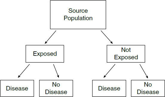
The difference between cohort and case-control studies is that cohort studies measure and compare health outcomes (such as the presence or absence of a particular disease)26 in the exposed and unexposed groups (or between individuals that experienced different levels of exposure), while case-control studies measure and compare the frequency (or level) of exposure in the group with the disease (the cases) and the group without the disease (the controls). In a cohort study, the subjects’ exposure is determined before their health status (see Figure 1). The risk of disease among the exposed can then be compared with the risk of disease among the unexposed. In a case-control study, the health status is determined first. The odds that someone with the disease was exposed to a suspected agent can then be compared with the odds that someone without the disease was similarly exposed. As for most epidemiologic studies, these study designs aim to determine if there is an association between exposure to an agent and a health outcome and the strength (magnitude) of that association.
23. See David A. Freedman, Editorial: Oasis or Mirage?, 21 Chance no. 1, 59–61 (2008), https://doi.org/10.1080/09332480.2008.10722888.
24. Sometimes, for practical reasons, the source population from which the researcher draws study subjects is not exactly the same as the population about which the researcher wants to make inferences, in which case the term target population is used to distinguish the population about which inferences are made from the source population.
25. See section titled “Ecological Studies” below. For thumbnail sketches on all types of epidemiologic study designs, see Brian L. Strom, Basic Principles of Clinical Epidemiology Relevant to Pharmacoepidemiologic Studies, in Pharmacoepidemiology 44, 50–55 (Brian L. Strom et al. eds., 6th ed. 2020), https://doi.org/10.1002/9781119413431.ch3.
26. Although epidemiologists refer generally to “health outcomes,” some disease is usually the health outcome of interest in the types of court cases in which epidemiologic research plays an important role. See supra discussion, note 1.
Cohort Studies
In cohort studies, researchers define a study population without regard to the participants’ disease status. The cohort may be defined in the present and followed forward into the future (prospectively), in which case they are known as prospective, longitudinal, or follow-up studies. Alternatively, a cohort study may be constructed retrospectively as of some time period in the past and followed from that historical time toward the present. In cohort studies, there is usually a group that is unexposed and another that is exposed, or several groups with different levels of exposure (including, in appropriate cases, a group with no exposure). Exposure may also be measured continuously (e.g., blood lead levels). In a prospective study, individuals are enrolled and followed over time, during which exposure and subsequent health outcomes are measured, while in a retrospective study, the researcher will obtain data on past exposure from available records, samples, questionnaires, or other evidence.27 So, for a study aiming to determine the association between an exposure and the occurrence of a disease, a researcher would compare the proportion of unexposed individuals who have the disease with the proportion of exposed individuals who have the
27. Sometimes in retrospective cohort studies, the researcher gathers historical data about exposure and disease outcome of a cohort. See Harold A. Kahn, An Introduction to Epidemiologic Methods 39–41 (1983); Mark A. Klebanoff & Jonathan M. Snowden, Historical (Retrospective) Cohort Studies and Other Epidemiologic Study Designs in Perinatal Research, 219 Am. J. Obstetrics & Gynecology 447 (2018), https://doi.org/10.1016/j.ajog.2018.08.044. Irving Selikoff, in his seminal study of asbestotic disease in insulation workers, included several hundred workers who had died before he began the study. Selikoff was able to obtain information about exposure from union records and information about disease from hospital and autopsy records. Irving J. Selikoff et al., The Occurrence of Asbestosis Among Insulation Workers in the United States, 132 Ann. N.Y. Acad. Sci. 139, 143 (1965), https://doi.org/10.1111/j.1749-6632.1965.tb41097.x.
disease.28 If the exposure causes the disease, the researcher would expect a greater proportion of the exposed individuals to develop the disease than the unexposed individuals.29 For a health outcome that is measured continuously, such as intelligence quotient (IQ) or blood pressure, the researcher could compare the average of these outcomes among the exposed and unexposed. If exposure is measured as a continuous rather than a dichotomous variable—for example, if all study subjects were exposed to some radiation from a nuclear accident but the degree of exposure was lower for those farther away from the accident—the researcher could examine the association between the extent of exposure and the health outcome.
One advantage of the cohort study design is that the temporal relationship between exposure and disease can often be established more readily than in other study designs. By tracking people who initially have not been diagnosed with the disease, the researcher can determine the time of disease onset (or diagnosis) and its relation to exposure. This temporal relationship is critical to the question of causation, because exposure must precede disease onset for exposure to have caused the disease.
As an example, in 1950 a cohort study was begun to determine whether uranium miners exposed to radon were at increased risk of death due to lung cancer as compared with nonminers. The study group (also referred to as the exposed cohort) consisted of 3,400 underground miners. The control group or unexposed cohort (which need not be the same size as the exposed cohort) comprised nonminers from the same geographic area. Members of the exposed cohort were examined every three years, and the degree of this cohort’s exposure to radon was measured from samples taken in the mines. Ongoing testing for radioactivity and periodic medical monitoring of lungs permitted the researchers to examine whether disease was linked to prior work exposure to radiation and allowed them to discern the relationship between exposure to radiation and disease. Exposure to radiation was associated with the development of lung cancer in uranium miners.30
The cohort design often is used in occupational studies such as the one just discussed. But because the design is not experimental, the investigator has no control over what other exposures a worker in the study may have had. Hence, an increased risk of disease among the exposed group may be caused by agents other than the exposure of interest. A researcher planning a study must attempt to
28. See Table 1, infra, in the section titled “Relative Risk.”
29. Researchers often examine the rate of disease or death in the exposed and control groups. The rate of disease or death entails consideration of the number developing disease within a specified period. All smokers and nonsmokers will, if followed for 100 years, die. Smokers will die at a greater rate than nonsmokers in the earlier years.
30. This example is based on a study description in Abraham M. Lilienfeld & David E. Lilienfeld, Foundations of Epidemiology 237–39 (2d ed. 1980). The original study is Joseph K. Wagoner et al., Radiation as the Cause of Lung Cancer Among Uranium Miners, 273 NEJM 181 (1965), https://doi.org/10.1056/NEJM196507222730402.
identify factors (called confounders) other than the exposure that may be related to exposure and may be responsible for the increased risk of disease. We discuss this problem (which is not limited to cohort studies) below in the “Confounding Bias” section. If data are gathered about potential confounders, the researcher generally uses statistical methods31 to estimate an association that is independent of these factors. Evaluating whether the association is causal involves additional analysis, as discussed below in the “General Causation” section.
Case-Control Studies
In case-control studies, the researcher begins with a group of individuals who have a disease (cases) and then selects a similar group of individuals who do not have the disease (controls). Controls should come from the same source population as the cases. The researcher then compares the extent of exposure in the two groups. For example, researchers might use employment records or questionnaire responses to determine whether and to what extent each study subject was exposed to the agent of interest, or researchers might measure biomarkers in the cases and controls to infer their exposure history. If a certain exposure is associated with the disease, a higher odds of exposure would be observed among the cases than among the controls (see Figure 2). Because researchers employing this research design often (though not always) gather historical information about exposure to an agent in the case and control groups, case-control studies have sometimes, but less precisely, been referred to as “retrospective studies.”32
For example, in the late 1960s, doctors in Boston were confronted with an unusual number of young female patients with vaginal adenocarcinoma. Those

31. See generally Daniel L. Rubinfeld & David Card, Reference Guide on Multiple Regression and Advanced Statistical Models, in this manual; Kaye & Stern, supra note 16, “Statistical Models” (discussing difficulties of multiple regression).
32. As described, the design of a case-control study is inherently retrospective rather than prospective. But other types of epidemiologic studies, including some cohort studies, may also be retrospective. See Strom, supra note 25 and accompanying text.
patients became the cases in a case-control study (because they had the disease in question). Controls who did not have the disease were selected based on their being born in the same hospitals and at the same time as the cases. The cases and controls were compared for exposure to agents that might be responsible, and researchers found maternal ingestion of diethylstilbestrol (DES), a drug prescribed to prevent miscarriage and premature delivery, in all but one of the cases but none of the controls.33
An advantage of the case-control study is that it usually can be completed in less time and with less expense than a cohort study. Case-control studies are also particularly useful in the study of rare diseases, because if a cohort study were conducted, a large group of individuals would have to be studied in order to observe the development of a sufficient number of cases for statistical analysis.34 A number of potential limitations of case-control studies are discussed in the section below titled “Biases.”
Cross-Sectional Studies
A third type of observational study is a cross-sectional study. In this type of study, for each study participant the presence of both the exposure of interest and the health outcome of interest is assessed at a single point in time. Thus, cross-sectional studies reveal the prevalence (i.e., the presence at that particular time) of both exposure and disease but do not provide the disease incidence (i.e., the development of disease over time).35 A researcher interested in the association between a health outcome (e.g., IQ) and an exposure that is relatively consistent over time (e.g., blood lead levels from living in contaminated housing) might use a cross-sectional study design. However, because a cross-sectional study determines both exposure and disease in an individual at the same point in time, it may be impossible to establish the temporal relation between exposure and disease—that is, whether the exposure preceded the disease, which is necessary for drawing any causal inference. Indeed, cross-sectional studies may be
33. See Arthur L. Herbst et al., Adenocarcinoma of the Vagina: Association of Maternal Stilbestrol Therapy with Tumor Appearance in Young Women, 284 NEJM 878 (1971), https://doi.org/10.1056/NEJM197104222841604.
34. For example, to detect a statistically significant doubling of disease caused by exposure to an agent where the incidence of disease is 1 in 100 in the unexposed population would require sample sizes of 3,100 for the exposed and nonexposed groups for a cohort study, but only 177 for the case and control groups in a case-control study (see section titled “Sampling Error” below for a discussion of statistical significance). Harold A. Kahn & Christopher T. Sempos, Statistical Methods in Epidemiology 66 (1989). See also Kaye & Stern, supra note 16, “What Is the Standard Error?,” “What Is the Confidence Interval?,” and “Tests or Interval Estimates?”
35. See In re Deepwater Horizon Belo Cases, No. 3:19CV963-MCR-HTC, 2022 WL 17721595, at *10 (N.D. Fla. Dec. 15, 2022) (criticizing failure of expert to identify a study on which she relied as a cross-sectional study).
affected by reverse causation, in which the health outcome under study actually causes a change in exposure.36 Though more limited than cohort or case-control studies, cross-sectional studies can provide valuable leads to further directions for research, particularly when reverse causation can be ruled out based on other knowledge.37
Ecological Studies
Up to now, we have discussed studies in which data on both exposure and health outcome are obtained for each individual included in the study, although individual data are sometimes augmented by group-level information, such as data from census tracts. Other studies, called ecological studies, collect only aggregate data on groups as a whole. In ecological studies, rather than gathering information about individuals, researchers obtain and compare overall rates of disease or death (or other summary measure for continuous health outcomes) for different exposure groups.38
One type of ecological study compares exposure groups across geographic locations. For example, epidemiologists might compare disease rates among areas with more or less air pollution.39 When making such comparisons, epidemiologists may overlay data on demographic factors obtained from sources such as the American Community Survey. Epidemiologists may look at geospatial or temporal trends (which may identify so-called “clusters” of disease) to form hypotheses and research questions.40
Ecological studies may be useful to identify associations for further exploration, but they can rarely provide causal answers. We illustrate the difficulty of
36. For example, a cross-sectional study might find that disinfectant use is associated with greater odds of asthma, but could not distinguish whether disinfectants cause people to have asthma or whether having asthma causes people to use disinfectants.
37. For more information and references about cross-sectional studies, see David D. Celentano & Moyses Szklo, Gordis Epidemiology 154–57 (6th ed. 2018).
38. Studies may be conducted in which all members of a group or community are treated as exposed to an agent of interest (e.g., a contaminated water system) and disease status is determined individually. These studies should be distinguished from ecological studies.
39. See Jonah Lipsitt et al., Spatial Analysis of COVID-19 and Traffic-Related Air Pollution in Los Angeles, 153 Env’t Int’l 106531 (2021), https://doi.org//10.1016/j.envint.2021.106531.
40. For example, the observed emergence of a cluster of adverse events associated with the use of heparin, a longtime and widely prescribed anticoagulant, led to suspicions that some specific lot of heparin was responsible. The observed pattern led the Centers for Disease Control and Prevention to conduct a case-control study, which concluded that contaminated heparin manufactured by Baxter was responsible for the outbreak of adverse events. See David B. Blossom et al., Outbreak of Adverse Event Reactions Associated with Contaminated Heparin, 359 NEJM 2674 (2008), https://doi.org/10.1056/NEJMoa0806450; In re Heparin Prods. Liab. Litig., 803 F. Supp. 2d 712 (N.D. Ohio 2011).
using ecological studies to determine causality with the following hypothetical ecological study.
Suppose that researchers, interested in determining whether a high dietary-fat intake is associated with breast cancer, compared different countries in terms of their average fat intakes and their average rates of breast cancer. If countries with high average fat intake also tend to have high rates of breast cancer, the finding would suggest an association between dietary fat and breast cancer. However, such a finding would be far from conclusive, because it lacks particularized information about an individual’s exposure and disease status (i.e., whether an individual with high fat intake is more likely to have breast cancer).41 In addition to the lack of information about an individual’s intake of fat, the researcher does not know about the individual’s exposures to other agents (or other factors, such as a woman’s age when she first gave birth) that may also be responsible for the increased risk of breast cancer. This lack of information about each individual’s exposure to an agent and disease status can lead to an erroneous inference about the relationship between fat intake and breast cancer, a problem known as the ecological fallacy. The fallacy is assuming that, on average, the individuals in the study who have suffered from breast cancer consumed more dietary fat than those who have not suffered from the disease. This assumption may not be true. Nevertheless, the study is useful in that it identifies an area for further research: the fat intake of individuals who have breast cancer as compared with the fat intake of those who do not. Researchers who identify a difference in disease or death in an ecological study may follow up with a study of individuals.42
In another type of ecological study, epidemiologists may compare disease rates over time and focus on disease rates before and after a point in time when some event of interest took place. For example, after the once widely prescribed drug Bendectin was removed from the market, the rate of limb-reduction birth defects did not change, which suggested that Bendectin did not cause birth
41. For a discussion of the data on this question and what they might mean, see Kaye & Stern, supra note 16.
42. Some courts have admitted expert testimony that relied on the results of ecological studies. In Cook v. Rockwell Int’l Corp., 580 F. Supp. 2d 1071, 1095–96 (D. Colo. 2006), the plaintiffs’ expert conducted an ecological study in which he compared the incidence of two cancers among those living in a specified area adjacent to the Rocky Flats Nuclear Weapons Plant with other areas more distant. (The likely explanation for relying on this type of study is the time and expense of a study that gathered information about each individual in the affected area.) The court recognized that ecological studies are less probative than studies in which data are based on individuals but nevertheless held that this limitation went to the weight of the study. Plaintiffs’ expert was permitted to testify to causation, relying on the ecological study he performed. See also Mead v. Sec’y of Health & Hum. Servs., 2010 WL 892248, at *38 (Fed. Cl. Mar. 12, 2010) (“Because these studies examine trends in the aggregate rather than examining disease onset in exposed individuals, ecological studies are afforded less evidentiary weight in the medical community than controlled studies are.”).
defects.43 By contrast, researchers’ discovery that the timing of a dramatic increase in limb-reduction birth defects followed widespread use of the drug thalidomide supported the conclusion that thalidomide caused those defects.44
However, other than with such powerful agents as thalidomide, which increased the incidence of limb-reduction birth defects by several orders of magnitude, these secular-trend studies (also known as timeline studies) are less reliable and less able to detect modest causal effects than are the observational studies described above.45 Other factors that affect the measurement or existence of the disease, such as improved diagnostic techniques and changes in lifestyle or age demographics, may change over time. If those factors can be identified and measured, it may be possible to control for them with statistical methods. Of course, unknown factors cannot be controlled for in these or any other kinds of epidemiologic studies.
Genetic and Molecular Epidemiologic Studies
Epidemiology, like other fields of biological and medical science, has in recent decades been touched powerfully by advances in scientists’ ability to identify and study the molecular constituents of human cells, tissues, and organs. Perhaps the best-known of these advances is the development of genomics: the study of the human genome, the sequence of DNA bases arranged in chromosomes that form
43. See Wilson v. Merrell Dow Pharms., 893 F.2d 1149 (10th Cir. 1990) (affirming judgment entered for defendant on a jury verdict). In Wilson, the defendant introduced evidence showing total sales of Bendectin and the incidence of limb-reduction birth defects during the 1970–1984 period. In 1983, Bendectin was removed from the market, but the rate of limb-reduction birth defects did not change. The Tenth Circuit held that the district court correctly determined that the timeline data were admissible and the defendant’s expert witnesses could rely on those data in rendering their opinions. Id. at 1152–53. See also Siharath v. Sandoz Pharms. Corp., 131 F. Supp. 2d 1347 (N.D. Ga. 2001). In Siharath, the court took note of the absence of secular trend data to support plaintiff’s claim. After describing why several observational studies produced, at best, inconclusive results about any association between use of the lactation-suppressing drug Parlodel and the very rare complication of postpartum stroke, the court observed: “No evidence has been offered of an increase in postpartum strokes after the drug [Parlodel] was approved for suppression of lactation; no evidence has been offered of a decrease in postpartum strokes after the approval for suppression of lactation was withdrawn.” Id. at 1358.
44. Michael D. Green, Bendectin and Birth Defects 70–71 (1996) (describing how thalidomide’s teratogenicity was discovered after Dr. Widukind Lenz found a dramatic increase in the incidence of limb-reduction defects in Germany beginning in 1960).
45. See Graddy v. Sec’y of Health & Hum. Servs., No. 08-416V, 2017 WL 11286536, at **18–22 (Fed. Cl. Aug. 31, 2017) (finding that the expert witness’s ecological study on childhood autism prevalence and the introduction or increased doses of certain vaccines did not allow for a reliable evidentiary inference of causation regarding MMR II, varicella, and hepatitis A vaccines and autism).
the basis of heredity.46 But genomics is just one of several fields of large-scale research on categories of biological molecules and features, such as epigenomics,47 proteomics,48 and others. Rapid technological and computational improvements have increasingly facilitated “omics” studies that can be performed on a larger scale, at a lower cost, and in a shorter time.49
Variations in genes and other biochemical constituents across the population may be associated with the incidence of disease or the ability to metabolize an agent, and therefore can be subject to epidemiologic study. Genetic epidemiology assesses the genetic components that, perhaps in combination with environmental or other risk factors, contribute to the development or progression of disease in human populations.50 More generally, molecular epidemiology “joins an understanding of disease at a molecular level with population-based study designs and approaches.”51 The number of epidemiologic studies that include molecular and genetic factors is quickly increasing.52
Genetic and molecular epidemiologic studies add to epidemiology the ability to consider types of data that were previously unavailable. Where researchers previously could collect data only on the health outcome of interest, the exposure of interest, and relatively easily observed other potentially relevant traits
46. See Int’l Hum. Genome Sequencing Consortium, Initial Sequencing and Analysis of the Human Genome, 409 Nature 860 (2001), https://doi.org/10.1038/35057062. Genomics is contrasted to genetics by its scale: genetics is the study of the inheritance or effect of one gene or a relatively small number of genes; genomics is the study of the entire human genome or large portions of it.
47. Epigenetic factors are biochemical features or constituents that affect the extent to which genes are “turned on,” that is, expressed through synthesis of the proteins the genes encode. They have been described as an “extra layer of instructions that influences gene activity.” Gail P. A. Kauwell, Epigenetics: What It Is and How It Can Affect Dietetics Practice, 108 J. Am. Dietetic Ass’n 1056, 1056 (2008), https://doi.org/10.1016/j.jada.2008.03.003. Epigenomics has been defined as “[t]he study of epigenetic marks . . . on a genome-wide scale.” Pauline A. Callinan & Andrew P. Feinberg, The Emerging Science of Epigenomics, 15 Hum. Molecular Genetics R95, R96 (2006), https://doi.org/10.1093/hmg/ddl095.
48. Proteomics is the study of the proteome, the “complete set of proteins made by an organism.” Nat’l Cancer Inst., Proteomics, Dictionary of Cancer Terms, https://perma.cc/74G5-ZWNB; Proteome, id., https://perma.cc/ZQ79-HX5R.
49. See, e.g., Matthew K. Sigurdson et al., Redundant Meta-Analyses Are Common in Genetic Epidemiology, 127 J. Clinical Epidemiology 40, 46 (2020), https://doi.org/10.1016/j.jclinepi.2020.05.035 (“The advent of genomewide agnostic approaches and massive new biobanks and consortia has created a new paradigm for human genome epidemiology.”); Sara Goodwin et al., Coming of Age: Ten Years of Next-Generation Sequencing Technologies, 17 Nature Rev. Genetics 333, 333–37 (2016), https://doi.org/10.1038/nrg.2016.49 (describing gene sequencing technologies and stating that cost of sequencing a single genome had been reduced to about $1,000).
50. This description is closely paraphrased from John S. Witte & Duncan C. Thomas, Genetic Epidemiology, in Timothy L. Lash et al., Modern Epidemiology 963, 963 (4th ed. 2021), https://doi.org/10.1093/aje/kwj102.
51. Claire H. Pernar et al., Molecular Epidemiology, in Lash et al., supra note 50 at 935.
52. See, e.g., Muin J. Khoury et al., Genetic Epidemiology with a Capital E, Ten Years After, 35 Genetic Epidemiology 845 (2011), https://doi.org/10.1002/gepi.20634.
such as age or socioeconomic status, researchers may now also be able to collect information about the study subjects’ genotype or relevant cellular or molecular components. But adding genetic or molecular information about the study subjects does not somehow turn epidemiology from a population-based science into the study of individuals, any more than including information about the study subjects’ exposures and health outcomes did. Neither do genetic and molecular epidemiology constitute new types of epidemiologic study designs. Rather, they apply existing modes of epidemiologic study to genetic or molecular information. Thus, genetic and molecular epidemiologic studies employ various combinations of the study designs, such as cohort studies and case-control studies, described in the preceding subsection. Depending on the type of genetic or molecular data under study and the details of the study design, genetic and molecular epidemiologic studies are subject to the same sources of error that must be considered in designing and interpreting the results of any epidemiologic study.53
As with other epidemiologic studies, genetic and molecular epidemiology studies may be used to support or undermine claims of disease causation in litigation. Although commentators have long forecast that the output of genetic and molecular epidemiology would revolutionize causal proof, as of this writing few judicial opinions have addressed these types of studies, and it is far from clear that a revolution is in the offing. Nevertheless, it is increasingly likely that expert witnesses will rely on such studies in forming their opinions presented in courts.
In particular, genetic epidemiology may provide additional evidence of whether there is a causal connection between an environmental exposure and a disease at issue in litigation—either in a general sense or in the plaintiff’s specific instance. For example, a study found that maternal exposure to organophosphate insecticides was associated with shorter gestational duration only among infants who had a genetic variant that resulted in a slower elimination of these insecticides.54 Alternatively, genetic epidemiology may reveal associations between genetic variations and a plaintiff’s disease, raising the issue of whether or not a genetic variation may be a competing cause of the disease. This requires assessment of whether the gene–disease association is causal in a general sense, whether it acts independently of the exposure, and whether it is a competing cause in the plaintiff’s specific instance. The extreme, though not typical, example would be
53. Pernar et al., supra note 51, at 936 (emphasizing that although molecular epidemiology involves new “omics” technologies, “molecular epidemiology can only contribute valid and reproducible findings if epidemiologists critically integrate core methodological concepts of epidemiology”); id. at 947–52 (discussing usefulness of various epidemiologic study designs in molecular epidemiology research).
54. Kim G. Harley et al., Association of Organophosphate Pesticide Exposure and Paraoxonase with Birth Outcome in Mexican-American Women, PLoS One 6(8):e23923 (2011), https://doi.org/10.1371/journal.pone.0023923.
a health outcome or disease entirely determined by genetics,55 as is the case with sickle cell anemia.56
Molecular epidemiology may also become relevant to causation disputes in ways that go beyond genetics. In molecular epidemiology studies, as one researcher described them, “risk factors, outcomes, confounders or effect modifiers are measured with biomarkers.”57 Parties may use these types of studies to support or undermine claims that a plaintiff was exposed to an alleged toxicant, that an exposure caused a plaintiff’s disease or otherwise affected the plaintiff’s biochemistry or physiology, or that the plaintiff suffers from a particular condition or disease. In particular, parties may attempt to rely on research that seeks to identify “signature” molecular markers of disease etiology, with the validity, sensitivity, and specificity of the purported signatures likely to be in dispute.58 For example, in several cases involving claims that exposure to benzene caused a plaintiff’s leukemia, courts have considered the significance of certain chromosome aberrations as possible biomarkers of exposure or effect.59
55. E.g., Bowen v. E.I. Du Pont de Nemours & Co., No. CIV.A. 97C-06-194 CH, 2005 WL 1952859 (Del. Super. Ct. June 23, 2005), aff’d, 906 A.2d 787 (Del. 2006) (discussing how a newly discovered test for a newly discovered genetic variant established that a genetic mutation rather than a toxic exposure was “the cause of” plaintiff’s condition).
56. The sickle cell trait is a well-known example of a genetically determined condition. See Muin J. Khoury & Janice S. Dorman, Genetic Disease, in Molecular Epidemiology 365, 370 (Paul A. Schulte & Frederica P. Perera eds., 1993).
57. Paolo Boffetta, Biomarkers in Cancer Epidemiology: An Integrative Approach, 31 Carcinogenesis 121, 125 (2010), https://doi.org/10.1093/carcin/bgp269. Confounders are discussed in the section titled “Biases” below and effect modifiers are discussed in the section titled “Effect Modification” below.
58. Validity, in this context, refers to the degree to which the measurement of the “signature” marker measures what it purports to measure, as well as to whether the selected marker is generalizable from the study that derived it to the case in which it is being used. Sensitivity refers to the ability of an “etiologic signature” to identify true causal cases, i.e., to avoid false negatives. Specificity refers to the ability of an etiologic signature to identify false causal cases, i.e., to avoid false positives. The absence of a highly sensitive etiologic marker would be stronger evidence against causation than would be the absence of a less sensitive marker. The presence of a highly specific etiologic marker would be stronger evidence for causation than would be the presence of a less specific marker. See Steve C. Gold, When Certainty Dissolves into Probability: A Legal Vision of Toxic Causation for the Post-Genomic Era, 70 Wash. & Lee L. Rev. 237, 265–76 (2013) (discussing these concepts); see also infra Glossary of Terms.
59. E.g., Henricksen v. ConocoPhilips Co., 605 F. Supp. 2d 1142, 1149–50 (E.D. Wash. 2009) (noting absence in plaintiff of chromosomal aberrations found more frequently in toxicant-induced acute myelogenous leukemia than in idiopathic cases); Hendrian v. Safety-Kleen Sys., Inc., No. 08-14371, 2014 WL 1464462, at *7 (E.D. Mich. Apr. 15, 2014) (describing plaintiff’s expert’s testimony that presence of chromosomal aberrations indicated prior exposure to benzene); Harris v. KEM Corp., No. 85 CIV. 2127 (WK), 1989 WL 200446, at *3–*5 (S.D.N.Y. Dec. 2, 1989) (denying defendant’s motion for summary judgment where plaintiff’s expert testified that plaintiff’s leukemia had chromosomal aberrations consistent with benzene exposure).
Epidemiologic and Toxicologic Studies
In addition to observational epidemiology, toxicology models based on animal studies (in vivo) may be used to determine toxicity in humans.60 Animal studies have a number of advantages. They can be conducted as true experiments by assigning exposure at random and carefully controlling and measuring exposure. Animal studies can avoid the other problems that human epidemiology studies confront such as confounding61 by, for example, genetics, social factors, or nutrition; participant refusal, non-compliance, or loss to follow-up; and certain ethical issues including those involving certain subpopulations, such as pregnant women and children. Test animals can be sacrificed and their tissues examined, which may improve the accuracy of disease assessment.62 Animal studies often provide useful information about pathological mechanisms and play a complementary role to epidemiology by assisting researchers in framing and assessing the plausibility of hypotheses.
Animal studies have two significant disadvantages, however. First, animal study results must be extrapolated to another species—human beings—and differences in absorption, metabolism, and other factors may result in interspecies variation in responses. For example, one powerful human teratogen, thalidomide, does not cause birth defects in most rodent species.63 Similarly, some known teratogens in animals are not believed to be human teratogens.64 The second difficulty with inferring causation in humans based on animal studies is that such studies often use doses that are substantially higher than concentrations to which humans are exposed. This may require the estimation of dose–response relationships for lower doses that have not been tested in order to establish a dose at which no effect is expected. For many agents, such no-effect thresholds may
60. For an in-depth discussion of toxicology, see David L. Eaton et al., Reference Guide on Toxicology, in this manual.
61. See section titled “Effect Modification” below.
62. Ethical considerations against deliberately exposing humans to agents thought harmful, see supra note 18, have in the past not been thought to prohibit animal experimentation. Contemporary concern for the ethical treatment of animals used in research is reflected in a number of statutory and regulatory provisions. See, e.g., 15 U.S.C. § 2603(h)(1) (2022) (amended Toxic Substances Control Act requires Environmental Protection Agency to “reduce and replace, to the extent practicable, scientifically justified, and consistent with the policies of [the Act], the use of vertebrate animals in the testing of chemical substances and mixtures”); Nat’l Insts. Health, Animal Care & Use in the Intramural Research Program, NIH Policy Manual § 3040-2 (Mar. 18, 2022), available at https://perma.cc/9LW3-QJBQ; id. Appendix 1 (listing applicable statutes, regulations, standards, and policies).
63. Phillip Knightley et al., Suffer the Children: The Story of Thalidomide 271–72 (1979).
64. In general, it is often difficult to confirm that an agent known to be toxic in animals is safe for human beings. See Ian C.T. Nisbet & Nathan J. Karch, Chemical Hazards to Human Reproduction 98–106 (1983); Int’l Agency for Research on Cancer, Interpretation of Negative Epidemiological Evidence for Carcinogenicity (Nicholas J. Wald & Richard Doll eds., 1985) [hereinafter IARC (Wald & Doll)].
not be known or may not exist.65 Thus, inference conducted solely on the basis of animal studies is fraught with considerable uncertainty.66
Toxicologists also use in vitro methods, in which human or animal tissue or cells are grown in laboratories and are exposed to certain substances. While useful, the problem with this approach is also extrapolation—whether one can generalize the findings from the artificial setting of tissues in laboratories to whole human beings.67
Often toxicologic studies are the only or best available evidence of toxicity.68 Epidemiologic studies are difficult, time-consuming, expensive, and
65. See infra text accompanying footnotes 235–37.
66. See Soldo v. Sandoz Pharms. Corp., 244 F. Supp. 2d 434, 466 (W.D. Pa. 2003) (quoting the first edition of this reference guide); see also Gen. Elec. Co. v. Joiner, 522 U.S. 136, 143–45 (1997) (holding that the district court did not abuse its discretion in excluding expert testimony on causation based on expert’s failure to explain how animal studies supported expert’s opinion that agent caused disease in humans).
67. For a further discussion of these issues, see Eaton et al., supra note 60, “Extrapolation from Animal (In Vivo) and Cell (In Vitro) Research to Humans.” A number of courts have grappled with the role of animal studies in proving causation in a toxic substance case. One line of cases takes a very dim view of their probative value. For example, in Johnson v. Arkema, Inc., 685 F.3d 452 (5th Cir. 2012), the appellate court concluded that the district court did not abuse its discretion in discounting an animal study because “studies of the effects of chemicals on animals must be carefully qualified in order to have explanatory potential for human beings.” Id. at 463 (quoting Allen v. Pennsylvania Eng’g Corp., 102 F.3d 194, 197 (5th Cir. 1996)). See also Becnel v. BP Expl. & Prod., Inc., No. CV 17-1758-SDD-EWD, 2021 WL 4444723, at *2 (M.D. La. Sept. 28, 2021) (noting that relying on animal studies, in the absence of epidemiologic studies, is . . . “of very limited usefulness”) (quoting Brock v. Merrell Dow Pharms., Inc., 874 F.2d 307, 313 (5th Cir. 1989)); In re Mirena IUD Prod. Liab. Litig., 169 F. Supp. 3d 396, 445 (S.D.N.Y. 2016) (holding that the expert’s reliance on animal studies, without a sound basis for extrapolating these studies to humans, is inadmissible). Other courts have been more amenable to the use of animal toxicology in proving causation. See Metabolife Int’l, Inc. v. Wornick, 264 F.3d 832, 842 (9th Cir. 2001) (holding that the lower court erred in per se dismissing animal studies, which must be examined to determine whether they are appropriate as a basis for causation determination); see also In re Paoli R.R. Yard PCB Litig., 916 F.2d 829, 853–54 (3d Cir. 1990) (questioning the basis for the lower court’s exclusion of animal studies and remanding for further development of the record); Drake v. Allergan, Inc., 2014 WL 12718976, at *1 (D. Vt. Oct. 23, 2014) (“The Court is mindful that animal studies present certain risks but these risks are not sufficient to exclude them categorically, especially where there is other evidence of causation as is the case here.”). The Third Circuit in a subsequent opinion in Paoli observed:
[I]n order for animal studies to be admissible to prove causation in humans, there must be good grounds to extrapolate from animals to humans, just as the methodology of the studies must constitute good grounds to reach conclusions about the animals themselves. Thus, the requirement of reliability, or “good grounds,” extends to each step in an expert’s analysis all the way through the step that connects the work of the expert to the particular case. In re Paoli R.R. Yard PCB Litig., 35 F.3d 717, 743 (3d Cir. 1994); see also Cavallo v. Star Enter., 892 F. Supp. 756, 761–63 (E.D. Va. 1995) (courts must examine each of the steps that lead to an expert’s opinion), aff’d in part and rev’d in part, 100 F.3d 1150 (4th Cir. 1996).
68. The International Association for Research on Cancer (IARC), a well-regarded international public health agency, evaluates the human carcinogenicity of various agents. In doing so,
sometimes—when it is difficult to accurately measure exposure, or when the exposure or the disease is extremely rare—virtually impossible to perform.69 Consequently, epidemiologic studies do not exist for a large array of environmental agents. Where both toxicologic and epidemiologic studies are available, no universal rules exist for how to reconcile them.70 Researchers often employ
IARC obtains, evaluates, and synthesizes all of the relevant evidence, including animal studies as well as any human studies. IARC then publishes a monograph containing that evidence, IARC’s analysis, and a categorical assessment of the likelihood an agent is carcinogenic. In a preamble to each monograph, IARC explains what each of the categorical assessments means. IARC may classify a substance as “probably carcinogenic to humans” solely on the basis of the strength of animal studies. Int’l Agency for Research on Cancer, Human Papillomaviruses, 90 Monographs on Evaluation of Carcinogenic Risks to Humans 9–10 (2007), https://perma.cc/J52S-ELWH [hereinafter IARC Papillomaviruses]. When IARC monographs are available, courts generally recognize them as authoritative. See Hardeman v. Monsanto Co., 997 F.3d 941, 967 (9th Cir. 2021) (affirming lower court’s admission of IARC categorization of glyphosate as “a probable carcinogen”), cert. denied, 142 S. Ct. 2834 (2022). But IARC has only conducted evaluations of a fraction of potentially carcinogenic agents, and many suspected toxic agents cause effects other than cancer. See IARC, Revised Preamble for the IARC Monographs (2021), available at https://perma.cc/XXY4-7DKF.
69. Thus, in a series of cases involving Parlodel, a lactation suppressant for mothers of newborns, efforts to conduct an epidemiologic study of its effect on causing strokes were stymied by the infrequency of such strokes in women of child-bearing age. See, e.g., Brasher v. Sandoz Pharms. Corp., 160 F. Supp. 2d 1291, 1297 (N.D. Ala. 2001); see also In re Tylenol (Acetaminophen) Mktg., Sales Pracs. & Prods. Liab. Litig., No. 2:12-CV-07263, 2016 WL 3997046, at *7 (E.D. Pa. July 16, 2016) (in series of cases involving liver damage from use of acetaminophen (Tylenol) at or above the suggested dosage, efforts to conduct an epidemiological study of Tylenol’s effect on causing acute liver failure (ALF) were stymied by the rarity of drug-induced ALF). In other cases, a plaintiff’s exposure to an overdose of a drug may be unique or nearly so. See Zuchowicz v. United States, 140 F.3d 381 (2d Cir. 1998).
70. See IARC (Wald & Doll), supra note 64 (identifying several substances and comparing animal toxicology evidence with epidemiologic evidence). One explanation for the conflicting judicial treatment of toxicological studies of animals, see supra note 67, may be that when there is a substantial body of epidemiologic evidence that addresses the causal issue, courts find that animal toxicology has much less probative value. That was the case, for example, in several Bendectin cases. E.g., Turpin v. Merrell Dow Pharms., Inc., 959 F.2d 1349, 1359 (6th Cir. 1992); Brock v. Merrell Dow Pharms., Inc., 874 F.2d 307, 313; see also In re Paoli R.R. Yard PCB Litig., No. 86-2229, 1992 U.S. Dist. LEXIS 16287, at *16 (E.D. Pa. 1992) (excluding evidence of or based on animal studies linking PCB exposure to various health effects). Where epidemiologic evidence is not available, animal toxicology may be thought to play a more prominent role in resolving a causal dispute. See Michael D. Green, Expert Witnesses and Sufficiency of Evidence in Toxic Substances Litigation: The Legacy of Agent Orange and Bendectin Litigation, 86 Nw. U. L. Rev. 643, 680–82 (1992) (arguing that plaintiffs should be required to prove causation by a preponderance of the available evidence). For another explanation of the Bendectin cases as well as other toxic tort case clusters, see Gerald W. Boston, A Mass-Exposure Model of Toxic Causation: The Content of Scientific Proof and the Regulatory Experience, 18 Colum. J. Env’t L. 181 (1993) (arguing that epidemiologic evidence should be required in mass-exposure cases but not in isolated-exposure cases). See also IARC Papillomaviruses, supra note 68; Eaton et al., supra note 60, “Toxicology and Epidemiology.” The U.S. Supreme Court, in General Electric Co. v. Joiner, 522 U.S. 136, 144–45 (1997), suggested that there is no categorical rule for toxicologic studies, observing, “[W]hether animal studies can ever be a proper foundation for an expert’s opinion [is] not the issue. . . . The [animal] studies were so dissimilar to
an approach that considers the overall weight of evidence, that is, all of the relevant scientific evidence that addresses the question of interest.71 This methodology entails making a judgment about causation after carefully assessing the results, validity, and consistency of each epidemiologic and toxicologic study.72
Interpreting the Results of an Epidemiologic Study
Epidemiologists are ultimately interested in whether a causal link exists between an agent and a disease. However, the first question an epidemiologist generally addresses is whether an association is observed between exposure to the agent and disease. An association between exposure to an agent and disease is observed when disease occurs more frequently (or less frequently) when exposure exists than when exposure is absent.73 Although a causal relation is one possible explanation for an observed association between an exposure and a disease, an association does not necessarily mean that there is a cause–effect relation. Interpreting the meaning of an observed association is discussed below.74
the facts presented in this litigation that it was not an abuse of discretion for the District Court to have rejected the experts’ reliance on them.”
71. The methodology relies on expert scientific judgment to evaluate and weight the available evidence in order to reach the best conclusion. See Douglas L. Weed, Weight of Evidence: A Review of Concept and Methods, 25 Risk Analysis 1545 (2005), https://doi.org/10.1111/j.1539-6924.2005.00699.x. A number of courts have endorsed weight of evidence as a reliable methodology. See, e.g., In re Deepwater Horizon Belo Cases, No. 3:19CV963-MCR-HTC, 2022 WL 17721595, at *19 (N.D. Fla. Dec. 15, 2022) (stating that “weight of the evidence approach to analyzing causation can be considered reliable, provided the expert considers all available evidence carefully and explains how the relative weight of the various pieces of evidence led to his conclusion”) (quoting In re Abilify (Aripiprazole) Prods. Liab. Litig., 299 F. Supp. 3d 1291, 1311 (N.D. Fla. 2018)). As the court in In re Zantac (Ranitidine) Prod. Liab. Litig., 644 F. Supp. 3d 1075, 1168 (S.D. Fla. 2022), cogently observed: “Due to the ‘substantial judgment’ required of an expert in following this approach, it is crucial that the expert describe each step in the process by which he gathered and assessed the relevant scientific evidence” (quoting Abilify, supra, 299 F. Supp. at 1311)). When weight of evidence methodology is employed by a testifying expert, a critical step is adequately taking into account evidence contrary to the expert’s opinion. See Norris v. Baxter Healthcare Corp., 397 F.3d 878, 882 (10th Cir. 2005) (“We are simply holding that where there is a large body of contrary epidemiological evidence, it is necessary to at least address it with evidence that is based on medically reliable and scientifically valid methodology.”); Zantac, supra, at *129 (“a plaintiff’s expert must address epidemiological evidence that is inconsistent with his or her causation opinions”).
72. See sections titled “Statistical Power” and “General Causation” below.
73. A negative association implies that the agent has a protective or curative effect. Because the concern in toxic substances litigation is whether an agent caused disease, this reference guide focuses on positive associations.
74. See section titled “General Causation” below.
This section begins by describing the ways of expressing the existence and strength of an association between exposure and disease or health outcome. It then proceeds to address sources of error that may produce an incorrect or skewed association, including random chance (sampling error) and non-random or systematic error (bias). Systematic error may result, for example, from inaccuracies in ascertaining health and exposure, from the manner of selecting those studied and information about them, or from confounding bias. This section also describes the statistical methods epidemiologists use to evaluate the importance of, and to address, these potential sources of error with respect to whether an association is real.
The strength of an association between exposure and a health outcome can be stated in various ways. For categorical outcomes, such as the occurrence of a disease, measures often employed include relative risk, odds ratio, attributable risk, or standardized mortality (or morbidity) ratio.75 For continuous outcomes, such as IQ, researchers use other measures to describe the relationship between exposure and outcome. For example, statistical methods can be used to estimate a regression coefficient (sometimes called a beta coefficient) that represents the mean change in an outcome for a unit change in the level of exposure.76 Regardless of the type of health outcome studied or the particular measure of association used, each of these measurements of association examines the degree to which the risk of an adverse health outcome changes with exposure to an agent in a population of individuals.
75. These are the type of health outcomes, and thus the measures of association, most commonly at issue in litigation. See, e.g., In re Roundup Prods. Liab. Litig., 390 F. Supp. 3d 1102, 1120 n.18 (N.D. Cal. 2018) (identifying, explaining, and comparing relative risk and odds ratio); In re Lipitor (Atorvastatin Calcium) Mktg., Sales Pracs. & Prods. Liab. Litig., No. MDL214MN02502RMG, 2016 WL 827067, at *3 (D.S.C. Feb. 29, 2016) (discussing expert’s selection of method to express magnitude of association from among relative risk, odds ratio, and risk difference). The Glossary of Terms infra defines two additional measures of strength of association for categorical outcomes: hazard ratio (see Cooper v. Takeda Pharms. Am., Inc., 191 Cal. Rptr. 3d 67, 73–74, 78–79 (Cal. App. 2015) (describing expert testimony that defined and gave examples of hazard ratios)) and risk difference. A risk difference is the difference between the proportion of disease in those exposed to the agent and the proportion of disease in those who were unexposed. Thus, in the example given in the section titled “Relative Risk” below, the proportion of disease in those exposed is 40/100, the proportion of disease in the unexposed is 20/100, and the risk difference is 20/100 (40/100 minus 20/100). The risk difference is related to the attributable proportion of risk, another measure of association that is addressed below in the section titled “Attributable Risk.”
76. To estimate the association between an exposure and a continuous outcome, researchers compute beta coefficients, which are derived from standard multiple regression statistical analysis. See infra Glossary of Terms (defining beta coefficient). For more information on beta coefficients, see Rubinfeld & Card, supra note 31, “Appendix.” Court opinions discussing epidemiology have not, to date, addressed beta coefficients.
Relative Risk
A commonly used approach for expressing the association between an agent and disease in cohort studies is the relative risk (RR).77 It is defined as the ratio of the probability of disease in a group of exposed individuals (Re in Table 1 and the equation below) to the probability of disease in a group of unexposed individuals (Ru in Table 1 and the equation below). Consider the information a researcher would obtain in conducting a cohort study as depicted in Table 1.
Table 1. Cross Tabulation of Exposure by Disease Status
| No Disease | Disease | Totals | Risk of Disease | |
|---|---|---|---|---|
| Not Exposed | a | c | a + c | Ru = c/(a + c) |
| Exposed | b | d | b+ d | Re = d/(b+ d) |
The risk of disease is defined as the number of cases of disease that develop divided by the number of persons in the cohort under study.78 Thus, the risk expresses the probability that a member of the population will develop the disease.
For example, a researcher studies 100 individuals who are exposed to an agent and 200 individuals who are not exposed. After one year, 40 of the exposed individuals are diagnosed as having a disease, and 20 of the unexposed individuals also are diagnosed as having the disease. The relative risk of contracting the disease is calculated as follows:
- The risk of disease in the exposed individuals is 40 cases per 100 persons (40/100), or 0.4.
- The risk of disease in the unexposed individuals is 20 cases per 200 persons (20/200), or 0.1.
77. A relative risk cannot be calculated for a case-control study. An odds ratio is used instead to express the magnitude of any association found in such studies. See section titled “Odds Ratio” below.
78. Epidemiologists also use the concept of prevalence, which measures the existence of disease in a population at a given point in time, regardless of when the disease developed. Prevalence is expressed as the proportion of the population with the disease at the chosen time. See Celentano & Szklo, supra note 37, at 51–55.
- The relative risk is calculated as the ratio of the risk in the exposed group (0.4) divided by the risk in the unexposed group (0.1), or 4.0.
A relative risk of 4.0 indicates that the risk of disease in the exposed group is four times as high as the risk of disease in the unexposed group.79
Risk, as defined above (generally referred to as cumulative incidence), can only be estimated if all individuals are followed for an equal period of time. If the follow-up time period differs between individuals in a study, the incidence rate is used instead. Incidence rates account for the fact that individuals followed for a longer period of time have a greater opportunity to develop the disease under study than those followed for a shorter time. To compute an incidence rate, a researcher divides the number of observed cases by the cumulated person-time.80
In general, the relative risk can be interpreted81 as follows:
- If the relative risk equals 1.0, the risk in the group of exposed individuals is the same as the risk in the group of unexposed individuals.82 There is no association between exposure to the agent and disease.
- If the relative risk is greater than 1.0, the risk in the group of exposed individuals is greater than the risk in the group of unexposed individuals. There is a positive association between exposure to the agent and the disease, which may reflect a harmful effect of the agent in increasing the extent of disease.
- If the relative risk is less than 1.0, the risk in exposed individuals is less than the risk in unexposed individuals. There is a negative (or inverse) association between exposure to the agent and the disease, which could
79. See Celentano & Szklo, supra note 37, at 242–45; Magistrini v. One-Hour Martinizing Dry Cleaning, 180 F. Supp. 2d 584, 591 (D.N.J. 2002) (explaining the relationship between relative risk and the increased incidence of disease in the exposed group).
80. Person-time weights study participants by the amount of time those participants were observed and at risk for the disease. For example, one participant observed for one year is one person-year; one participant observed for two years is two person-years, etc. Two participants observed for one year each is also two person-years. The incidence rate is computed as the number of new cases of disease divided by the total person-time observed. See Celentano & Szklo, supra note 37, at 46–49.
81. For the sake of simplicity, this description refers only to relative risk. As noted in the immediately preceding text, if a cohort study follows different participants for different periods of time, the researcher computes an incidence rate ratio to determine if an association is observed. If an epidemiologic study reports an incidence rate ratio rather than a relative risk, the same interpretations as described in the text for relative risk would apply.
82. See Magistrini, 180 F. Supp. 2d at 591.
- reflect a protective or curative effect of the agent on risk of disease. For example, immunizations lower the risk of disease. Thus, immunizations are expected to be negatively associated with the diseases that they target.
Although relative risk is a straightforward concept, care must be taken in interpreting it. Whenever an association is uncovered, further analysis should be conducted to assess whether the association is causal or due to chance (random error) or bias (including confounding).83 These sources of error may also mask or skew a true association, resulting in a study that erroneously finds no association or overstates or understates the true association.
Epidemiologists often use relative risk as a measure of association in cohort studies. But researchers performing case-control studies cannot calculate a relative risk.84 Instead, epidemiologists conducting case-control studies compute a different measure of association: an odds ratio.
Odds Ratio
The odds ratio (OR) is similar to a relative risk in that it expresses in quantitative terms the association between exposure to an agent and a disease. It is a convenient way to estimate an association, most particularly in case-control studies, though it can also be calculated for a cohort study.85 The odds ratio approximates the relative risk when the disease is rare.86
In a case-control study, the odds ratio is the ratio of the odds87 that a case (one with the disease) was exposed to the odds that a control (one without the
83. See sections titled “Biases” and “Sampling Error” below.
84. A case-control study begins by examining a group of persons who already have the disease and another group of persons who do not have the disease. See section titled “Case-Control Studies” above. Because the number of cases and the number of controls are predetermined, the researcher cannot calculate the rate at which exposed and unexposed individuals in the study develop the disease. Lacking a rate or incidence of disease for both those exposed and those not exposed to the agent, a researcher cannot calculate a relative risk.
85. In a cohort study, the odds ratio is the ratio of the odds of a disease occurring when exposed to a suspected agent to the odds of the disease occurring when not exposed. An odds ratio can also be calculated for a cross-sectional study.
86. See Marcello Pagano & Kimberlee Gauvreau, Principles of Biostatistics 123 (3d ed. 2022). If the disease is not rare, the odds ratio is still valid to determine whether an association exists, but interpretation of its magnitude is less intuitive. For further detail about the odds ratio and its calculation, see Kahn & Sempos, supra note 34, at 47–56.
87. The odds of exposure is the ratio of those who were exposed to those who were not. Thus, from Table 2 infra, we can calculate the odds of exposure among the cases as a/c, and the odds of exposure among the controls as b/d.
disease) was exposed. Consider a case-control study, with results as shown schematically in a 2 × 2 table (Table 2):
Table 2. Cross Tabulation of Cases and Controls by Exposure Status
| Cases (with disease) | Controls (no disease) | |
|---|---|---|
| Exposed | a | b |
| Not exposed | c | d |
In a case-control study, the odds ratio OR is the odds that a case was exposed divided by the odds that a control was exposed. Looking at Table 2, this ratio can be calculated as:
Because we are multiplying two diagonal cells in the table and dividing by the product of the other two diagonal cells, the odds ratio is sometimes also called the cross-products ratio.
Consider the following hypothetical study: A researcher identifies 100 individuals with a disease who serve as cases and 100 people without the disease who serve as controls for her case-control study. Of the 100 cases (with disease), 40 were exposed to an agent under study and 60 were not. Among the control group, 20 people were exposed and 80 were not. The data can be presented in a 2 × 2 table (Table 3).
Table 3. Case-Control Study Outcome
| Cases (with disease) | Controls (no disease) | |
|---|---|---|
| Exposed | 40 | 20 |
| Not exposed | 60 | 80 |
The calculation of the odds ratio would be OR = (40/60)/(20/80) = 2.67.
If the disease is relatively rare in the general population (about 5% or less), the odds ratio is a good approximation of the relative risk. Thus, in our example, there is almost a tripling in the risk of the disease in those exposed to the agent relative to those who were not exposed.88
88. The odds ratio is usually more extreme (farther away from the null of 1.0) compared to the relative risk. In other words, if a relative risk is above 1.0, the odds ratio will tend to be larger; if a relative risk is below 1.0, the odds ratio will tend to be smaller. As the disease in question becomes more common, the difference between the odds ratio and the relative risk grows.
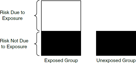
Attributable Risk
A frequently used measurement of risk is the attributable risk (AR), also called the attributable proportion of risk, the etiologic fraction, or the attributable risk percent. This measure represents the proportion of disease among exposed individuals that can be attributed to the exposure89 and therefore, if the association is causal, the proportion of disease that could potentially be prevented if exposure to the agent were eliminated (see Figure 3).90
The reason the odds ratio approximates the relative risk when the incidence of disease is small can be demonstrated by comparing the relative risk of a cohort study with its odds ratio. Referring to Table 1, the odds that the exposed group developed the disease is d/b; similarly, the odds that the unexposed group developed the disease is c/a; thus the odds ratio is (d/b)/(c/a) = ad/bc. Recall the relative risk would be [d/(b+d)] / [c/(a+c)] = [d(a+c)] / [c(b+d)]. Thus, when the incidence of disease is low, i.e., c and d are small in relation to a and b, the relative risk will approximate the odds ratio of ad/bc. See Celentano & Szklo, supra note 37, at 248–50.
If the disease is not rare, the relative risk may be estimated from the odds ratio. The formula for this estimate takes into account the prevalence of the disease among the unexposed (P0):
RR = OR/(1 – P0 + (P0 × OR)). In our example, if the disease had a 15% prevalence among the unexposed, the corresponding estimated relative risk would be 2.67/(1 – 0.15 + (0.15 × 2.67)) = 2.14. Note that, as described above, with a relatively high prevalence the numerical value of the odds ratio is farther from the null—in this case, greater than—the numerical value of the estimated relative risk. See Robert L. Grant, Converting an Odds Ratio to a Range of Plausible Relative Risks for Better Communication of Research Findings, 348 Brit. Med. J. f7540 (2014), https://doi.org/10.1136/bmj.f7450.
89. Kenneth J. Rothman et al., Measures of Effect and Measures of Association, in Lash, supra note 50, at 79, 93–97; see also Landrigan v. Celotex Corp., 605 A.2d 1079, 1086 (N.J. 1992) (illustrating that a relative risk of 1.55 corresponds to an attributable risk of approximately 35%).
90. Risk is not zero for the control group (those not exposed) when there are other causal chains that cause the disease that do not require exposure to the agent. For example, some birth defects are the result of genetic sources, which do not require the presence of any environmental agent. Also, some degree of risk in the control group may be the result of background exposure to
To determine the proportion of a disease that is attributable to an exposure, a researcher would need to know the risk of the disease in the exposed group and the risk of disease in the unexposed group. The attributable risk is
The attributable risk can be calculated using the example described in the section titled “Relative Risk.” Suppose a researcher studies 100 individuals who are exposed to a substance and 200 who are not exposed. After one year, 40 of the exposed individuals are diagnosed as having a disease, and 20 of the unexposed individuals are also diagnosed as having the disease.
- The risk of disease in the exposed group is 0.4 (40 persons with the disease out of 100 who are exposed).
- The risk of disease in the unexposed group is 0.1 (20 persons with the disease out of 200 who are not exposed).
- The proportion of disease in the exposed group that is attributable to the exposure is (0.4 −0.1)/0.4 = 0.75 or 75%.
This means that 75% of the disease in the exposed group is attributable to the exposure. We should emphasize here that attributable does not necessarily mean “caused by.” Up to this point, we have only addressed associations. Inferring causation from an association is addressed in the “General Causation” section below.
Internal and External Validity
Internal validity is concerned with whether the result of a study—an association, for example in an epidemiologic context—is an accurate assessment of the true association in the source population from which study participants were recruited. Various biases such as selection bias, confounding bias, and information bias (all discussed in the “Biases” section below) can affect internal validity. For example, if researchers interviewing participants in a case-control study know the participant’s disease status, they might subconsciously probe harder to find exposure to the agent in participants with the disease than in those without
the agent being studied. For example, nonsmokers in a control group may have been exposed to passive cigarette smoke, which is responsible for some cases of lung cancer and other diseases. See Ethyl Corp. v. EPA, 541 F.2d 1, 25 (D.C. Cir. 1976) (describing the difficulty of finding people without exposure to ubiquitously distributed agents). There are some diseases that do not occur without exposure to an agent; these are known as signature diseases.
disease. That would produce an inflated estimate of the real association and would compromise the study’s internal validity.91
External validity concerns whether the study results can be generalized to a different population. In the multidistrict litigation involving the drug phenylpropanolamine (PPA) used as an appetite suppressant, an epidemiologic study found an odds ratio of 16.58 for hemorrhagic stroke.92 The study was limited to individuals between the ages of 18 and 49 and, because of the paucity of men who had used PPA-containing appetite suppressants, the analysis was limited to women. In the litigation that followed, the court was faced with whether the study could be used to support causation for those under the age of 18, those over the age of 49, or men.93 That issue called into question the matter of external validity: the extrapolation of the study results to a population that was not a part of the study.
Sources of Error in Epidemiologic Studies
Incorrect study results can occur in a variety of ways. A study may find a positive association (relative risk greater than 1.0) when there is no true association. Or a study may erroneously find that that there is no association when in reality there is one. A study may also find an association when one truly exists, but the association found may be greater or less than the real association.
Two general categories of phenomena can cause erroneous associations: chance and bias. Before any inferences about causation are drawn from a study, the possible impact of these phenomena must be examined.94
The findings of a study may be the result of chance (also called sampling error or random error). In designing a study, the size of the sample can be
91. Any problem with a study’s internal validity would also affect the validity of any attempt to extrapolate the study’s results to a different population. As described in the next paragraph, this would create a problem of external validity in addition to the impact on internal validity.
92. See W.N. Kernan et al., Phenylpropanolamine and the Risk of Hemorrhagic Stroke, 343 NEJM 1826 (Dec. 21, 2000), https://doi.org/10.1056/NEJM200012213432501.
93. See In re Phenylpropanolamine (PPA) Prods. Liab. Litig., 289 F. Supp. 2d 1230, 1235 (W.D. Wash. 2003). There was additional evidence in the case that the court took into account; the description of the case in the text is a stylized one to concisely illustrate the idea of external validity.
94. See Philip Cole, Causality in Epidemiology, Health Policy, and Law, 27 Env’t L. Rep. 10279, 10285 (1997); DeLuca v. Merrell Dow Pharms., Inc., 911 F.2d 941, 955 (3d Cir. 1990) (recognizing and discussing random sampling error and then referring to other errors, such as systematic bias, that create as much or more error in the outcome of a study). See also Daniels-Feasel v. Forest Pharms., Inc., No. 17 CV 4188-LTS-JLC, 2021 WL 4037820, at *2 (S.D.N.Y. Sept. 3, 2021) (“Where a positive association is observed, its validity is assessed by evaluating the role of possible alternative explanations, such as chance, bias, or confounding.”). For a similar description of error in study procedure and random sampling, see Kaye & Stern, supra note 16, “What Inferences Can Be Drawn from the Data?”
increased to reduce (but not eliminate) the likelihood that a result may be due to chance. Statistical methods permit an assessment of the extent to which the results of a study may be due to chance, most often by computing a p-value and/or a confidence interval, which are closely related and are described in more detail in the “Sampling Error” section below.
Briefly, a calculated p-value is used to determine whether a study result is considered “statistically significant.” As described in more detail below, testing for statistical significance entails comparing the calculated p-value to a preselected threshold that enables an assessment of the role of random error in producing the study result. A result that is statistically significant is generally considered unlikely to be the result of chance, although any p-value threshold chosen is arbitrary.
A confidence interval provides information about the uncertainty (or precision) of an estimated measure of association (such as a relative risk or an odds ratio). A wide confidence interval suggests that chance is more likely to have an important impact on the estimate while a tight interval points to a likelihood of a smaller impact of chance and thus a more precise estimate.
We emphasize a point that those unfamiliar with statistical methodology frequently find confusing: That a study’s results are statistically significant says nothing about the magnitude of any association (i.e., the relative risk or odds ratio) or about the biological, clinical, or public health importance of the finding.95 Significant, as used with the adjective statistically, does not mean “big” or “important.” A large study may find a statistically significant relationship that is quite modest in magnitude—for example, a relative risk of 1.05. Another study may find an association that is quite large—say, a relative risk of 10.0 or even higher—yet is not statistically significant because of the potential for random error due to a small sample size.96 In short, statistical significance is not about the size of the risk associated with an exposure.97
95. See Modern Scientific Evidence, supra note 3, § 5.36 at 435 (“Statisticians distinguish between ‘statistical’ and ‘practical’ significance. . . .”); Cole, supra note 94, at 10282. Suppose a study finds a statistically significant risk of 1.05. If that association applies to a rare, easily managed side effect of a medication prescribed to treat a common, debilitating illness, the finding might be more a reason for relief than for concern. But if 1.05 is the relative risk of a common, serious illness associated with ubiquitous exposure to an air pollutant, the finding might be cause for great concern despite the small magnitude of the relative risk. Alternatively, suppose a study finds a relative risk of 10.0 that is not statistically significant. If that relative risk applies to an invariably fatal condition associated with a small number of exposures to a new chemical that is poised to enter widespread use, the finding might suggest a need for caution or further investigation.
96. To find small effects that are statistically significant, larger sample sizes are required. When effects are larger, fewer subjects are required to produce statistically significant findings. For further explanation, see the section titled “Sampling Error” below.
97. Understandably, some courts have been confused about the relationship between statistical significance and the magnitude of the association. See, e.g., Hyman & Armstrong, P.S.C. v. Gunderson, 279 S.W.3d 93, 102 (Ky. 2008) (conflating the magnitude of the association with
Bias also can produce error in the outcome of a study. In epidemiology, as in science generally, bias refers to methodological issues that skew a study’s results, with no connotation that a researcher has a subjective desire for, or interest in, a particular outcome. Bias encompasses any effect that tends to produce study results that differ from the true value in a systematic, rather than random, way. Thus, bias is also known as systematic error.
Epidemiologists attempt to minimize bias through their study designs, including data-collections protocols. Study designs are developed before researchers begin gathering data. However, some biases cannot be addressed at the design stage, and even the best-designed and conducted studies are likely to produce results that are biased to some extent. Consequently, after data collection is completed, statistical tools are often used to identify and correct for potential sources of bias. Epidemiologists may reanalyze a study’s data to correct for a bias identified in a completed study or to validate the analytical methods used.98 If correction (sometimes referred to as adjustment) for identified biases cannot be performed, epidemiologists can estimate whether the bias is likely to have inflated or diluted any association that may exist. Identification of uncorrected bias may enable an epidemiologist to make an assessment of the extent to which a study’s conclusions are valid. Common biases and how they may produce invalid results are described in the “Biases” section.
Sampling Error99
Before detailing the statistical methods used to assess sampling error (which we use synonymously with random error or chance), two concepts central to epidemiology and statistical analysis must be explained. Understanding these concepts should facilitate comprehension of the statistical methods. Epidemiologists often refer to true association (also called real association), which is the association that really exists between an agent and a disease in a given population and that might be found by a perfect (but nonexistent and impossible) study. The true association is a concept used in evaluating the results of a given study, even though its
whether it is statistically significant); In re Pfizer Inc. Sec. Litig., 584 F. Supp. 2d 621, 634–35 (S.D.N.Y. 2008) (confusing the magnitude of the effect with whether the effect was statistically significant); In re Joint E. & S. Dist. Asbestos Litig., 827 F. Supp. 1014, 1041 (S.D.N.Y. 1993) (concluding that any relative risk less than 1.50 is statistically insignificant), rev’d on other grounds, 52 F.3d 1124 (2d Cir. 1995). See generally Kaye & Stern, supra note 16, “Tests or Interval Estimates?”
98. E.g., Richard A. Kronmal et al., The Intrauterine Device and Pelvic Inflammatory Disease: The Women’s Health Study Reanalyzed, 44 J. Clinical Epidemiology 109 (1991), https://doi.org/10.1016/0895-4356(91)90259-C (a reanalysis of a study that found an association between the use of IUDs and pelvic inflammatory disease concluded that IUDs do not increase the risk of pelvic inflammatory disease).
99. For a bibliography on the role of statistical significance in legal proceedings, see Sanders, supra note 16, at 329 n.138.
value is unknown. By contrast, a study’s outcome will produce an observed association, which is known.
Formal procedures for statistical testing begin with the null hypothesis, which posits that there is no true association (i.e., a relative risk of 1.0) between exposure to the agent and the disease under study. Data are gathered and analyzed to see whether they disprove the null hypothesis.100 The data are subjected to statistical testing to assess the plausibility that any association found is a result of random error or whether, instead, the data support rejection of the null hypothesis.
The use of the null hypothesis for this testing should not be understood as the a priori belief of the investigator. When epidemiologists investigate an agent, it is usually because they hypothesize that the agent is a cause of some outcome. Nevertheless, in preparing their study designs, epidemiologists rely on the null hypothesis to test the plausibility that any association found in a study was the result of random error.101
False Positives and Statistical Significance
When a study results in a positive association (i.e., a relative risk greater than 1.0), epidemiologists try to determine whether that result represents a true association or is the result of random error. Random error can be illustrated by considering a fair coin (i.e., not modified to produce more heads than tails, or vice versa). On average, we would expect that coin tosses would yield half heads and half tails. But sometimes, a set of coin tosses might yield an unusual result—for example, six heads out of six tosses, an occurrence that, purely by chance, would result in less than 2% of a series of six tosses. In the world of epidemiology, sometimes the study findings, merely by chance, do not reflect the true relationships between an agent and outcome. Any single study—even a clinical trial—is in some ways analogous to a set of coin tosses, being subject to the play of chance. So, for example, even if the true relative risk (in the total population) were 1.0, an epidemiologic study might find an observed relative risk (in the study sample) greater than (or less than) 1.0 because of random error (i.e., chance).102 An erroneous conclusion that the null hypothesis is false (i.e., a conclusion that there is a different risk among those exposed to an agent relative to those that were
100. See, e.g., Daubert v. Merrell Dow Pharms., Inc., 509 U.S. 579, 593 (1993) (scientific methodology involves generating and testing hypotheses).
101. See DeLuca v. Merrell Dow Pharms., Inc., 911 F.2d 941, 945 (3d Cir. 1990); United States v. Philip Morris USA, Inc., 449 F. Supp. 2d 1, 706 n.29 (D.D.C. 2006); Stephen E. Fienberg et al., Understanding and Evaluating Statistical Evidence in Litigation, 36 Jurimetrics J. 1, 21–24 (1995), https://doi.org/10.1016/S0015-7368(91)73152-6.
102. See Magistrini v. One-Hour Martinizing Dry Cleaning, 180 F. Supp. 2d 584, 592 (D.N.J. 2002) (citing the second edition of this reference guide).
unexposed when no difference actually exists) owing to random error is called a false-positive error (also called a Type I error or alpha error).
Common sense leads one to believe that a large enough sample of individuals must be studied if the study is to identify a relationship that truly exists between exposure to an agent and a disease. Common sense also suggests that by enlarging the sample size (the size of the study group), researchers can form a more accurate conclusion and reduce the chance of random error in their results. Both statements are correct and can be illustrated by a test to determine if a coin is fair. A test in which a fair coin is tossed 1,000 times is more likely to produce close to 50% heads than a test in which the coin is tossed only 10 times. By contrast, it is far more likely that a test of a fair coin with 10 tosses will by chance come up with (for example) 80% heads than will a test with 1,000 tosses. With large numbers, the outcome of the test is less likely to be influenced by random error, and the researcher would have greater confidence in the inferences drawn from the data.103
Given a set of epidemiologic data, one might want to ask the straightforward, obvious question: What is the probability that an observed association reflects a real association that exists in the population from which the study subjects were drawn? But traditional statistical methods cannot answer this question.104 Instead, researchers compute “p-values” that address a related but very different question: Assuming there really is no association in the population—referred to as the null hypothesis—how probable is it that one would find an association in the study sample at least as large as the observed association?105
103. This explanation of numerical stability was drawn from Brief Amicus Curiae of Prof. Alvan R. Feinstein in Support of Respondent, Daubert v. Merrell Dow Pharms., Inc., No. 92-102, 1993 WL 13006284, at *12–*13 (U.S. Jan. 19, 1993). See also Allen v. United States, 588 F. Supp. 247, 417–18 (D. Utah 1984), rev’d on other grounds, 816 F.2d 1417 (10th Cir. 1987) (observing that although “[s]mall communities or groups of people are deemed ‘statistically unstable’” and “data from small populations must be handled with care[, it] does not mean that [the data] cannot provide substantial evidence in aid of our effort to describe and understand events”); Shi En Kim, Heads or Tails, Sci. Am., Jan. 2024, at 12 (explaining that if a coin were tossed a million times, an observed deviation of even one percent, such as 510,000 heads and 490,000 tails, would very likely result from a small but real bias in the coin).
104. For a discussion of Bayesian statistics, which under certain conditions can provide information about this probability, see infra text accompanying footnotes 120 and 178 and the entry “Bayesian analysis” in the Glossary of Terms.
105. This methodology, known as hypothesis testing, is one of the most counterintuitive techniques in statistics. See Modern Scientific Evidence, supra note 3, § 5.36 at 359 (“it is easy to mistake the p-value for the probability that there is no difference”).
The p-value for a given study does not provide a rate of error or even a probability of error for an epidemiologic study. In Daubert, 509 U.S. at 593, the Court stated that “the known or potential rate of error” should ordinarily be considered in assessing scientific reliability. Epidemiology, however, unlike some other methodologies—fingerprint identification, for example—does not permit
A p-value represents the probability that an association equal to or more extreme than (i.e., greater for a positive association or smaller for an inverse association) the observed association could be found if no association were in fact present, that is, if the null hypothesis were true.106 Thus, a p-value of 0.1 means that there is a 10% chance that, with no association being actually present in the population from which the study sample was drawn (i.e., under the null hypothesis), values at least as large as an observed relative risk above 1.0 could have occurred by random chance.107
The smaller the p-value, the less likely it is that the null hypothesis is true. Epidemiologists use a convention that the p-value must fall below some specified threshold, known as alpha or the significance level, for the results of the study to be considered statistically significant.108 Thus, an outcome is statistically significant when the observed p-value for the study falls below the preselected significance level.
Significance testing allows researchers to minimize false positive results. The most common significance level used in science is 0.05. As explained above, a p-value of 0.05 means that the probability of observing an association at least as large as that found in the study, when in truth there is no association, is
an assessment of its accuracy by testing against a known reference standard. A p-value provides information only about the plausibility of random Type I error given the study result, but the true relationship between agent and outcome remains unknown. A p-value provides no information about the plausibility of random Type II error (false negatives), which is discussed in the sections titled “False Negatives” and “Statistical Power” below. Moreover, a p-value provides no information about whether other sources of error exist and, if so, their magnitude. See sections titled “Biases” and “Conceptual Error” below. In short, for epidemiology, there is no way to determine a rate of error—even for the random error aspect of studies. See Kumho Tire Co. v. Carmichael, 526 U.S. 137, 151 (1999) (recognizing that for different scientific and technical inquiries, different considerations will be appropriate for assessing reliability); Cook v. Rockwell Int’l Corp., 580 F. Supp. 2d 1071, 1100 (D. Colo. 2006) (“Defendants have not argued or presented evidence that . . . there is, in fact, a method by which an overall ‘rate of error’ can be calculated for an epidemiologic study.”).
106. See also Kaye & Stern, supra note 16, “p-values, Significance Levels, and Hypothesis Tests” (the p-value reflects the implausibility of the null hypothesis).
107. Technically, a p-value of 0.1 means that if in fact there is no association, if the same study were to be repeated, 10% of such studies would be expected to yield an association the same as, or greater than, the one found in the study due to random error. The interpretation is similar for observed relative risks below 1.0: a p-value of 0.10 would represent a 10% chance that values equal or smaller would be due to random error. Note that the description here and in the text describes a “one-tailed” significance test. For an explanation of the distinction between one-tailed and two-tailed tests, see infra note 113.
108. Cook, 580 F. Supp. 2d at 1100–01 (discussing p-values and their relationship with statistical significance); Allen v. United States, 588 F. Supp. 247, 416–17 (D. Utah 1984), rev’d on other grounds, 816 F.2d 1417 (10th Cir. 1987) (discussing statistical significance and selection of a level of alpha); see also Sanders, supra note 16, at 343–44 (explaining alpha, beta, and their relationship to sample size); Developments in the Law—Confronting the New Challenges of Scientific Evidence, 108 Harv. L. Rev. 1481, 1535–36, 1540–46 (1995) [hereinafter Developments in the Law].
equal to 5%.109 When examining effect modification110 (such as when an association may differ by sex, social class, or genetics), epidemiologists usually use a higher p-value, e.g., a p-value of 0.10. This helps compensate for the fact that statistical power111 to detect effect modification is lower relative to that of the power to detect overall associations because stratifying by an effect modifier effectively reduces the sample size.112
Figure 4 presents a graphical depiction to assist understanding of significance testing. Under the null hypothesis, we assume that, if we performed many similar studies identical to the one for which we wish to estimate a p-value and graphed the frequency of their outcomes, we would expect to observe a normal (bell-shaped) distribution, with most results clustered near the null value (remember, we assume the null hypothesis) and only a few extreme results in the “tails,” far from the hypothesized null value, as depicted by the small shaded
109. This means that if one examined a large number of situations in which the true relative risk equals 1—meaning there is no association between any of the agents studied and the outcome of interest—on average 1 result in 20 nevertheless would show an association that is statistically significant at a .05 level. When researchers examine many possible associations that might exist in their data—known as data dredging—we should expect that even if there are no true causal relationships, those researchers will find statistically significant associations in 1 of every 20 associations examined. See Rachel Nowak, Problems in Clinical Trials Go Far Beyond Misconduct, 264 Sci. 1538, 1539 (1994), https://doi.org/10.1126/science.8202708. For an accessible discussion of this problem, see Andrew Gelman & Eric Loken, The Statistical Crisis in Science, 107 Am. Scientist (2014), https://doi.org/10.1511/2014.111.460.
In certain contexts, the sheer number of tests—and therefore the number of associations that would appear by chance—is so large that researchers apply much more stringent conventions for statistical significance. For example, researchers testing hundreds of thousands of genetic variations for association with disease typically accept as statistically significant only results that would appear by chance no more than once in every 20 million trials. See Laura Buzdugan et al., Assessing Statistical Significance in Multivariable Genome Wide Association Analysis, 32 Bioinformatics 1990, 1991 (2016) (“the multiple testing issue is resolved by applying a stringent significance threshold—most commonly 5 × 10⁻⁸”). Some researchers favor even greater stringency. Sara L. Pulit et al., Resetting the Bar: Statistical Significance in Whole-Genome Sequencing-Based Association Studies of Global Populations, 41 Genetic Epidemiology 145 (2016), https://doi.org/10.1002/gepi.22032 (arguing for significance levels ten to fifty times more stringent). Even in this context, the “cut points” chosen for statistical significance “are somewhat arbitrary and do not reflect the potential clinical or biological importance of associations, nor do they account for the cost of false negatives.” John S. Witte & Duncan C. Thomas, Genetic Epidemiology, in Lash et al., supra note 50, at 963, 970. For discussion of false negatives, see section titled “False Negatives” below.
110. See the section titled “Effect Modification” below for further explanation.
111. See the section titled “Statistical Power” below.
112. As explained infra at text accompanying footnote 172, researchers study effect modification using stratification—separating the study participants into subgroups (strata). For example, 200 participants in a study might be stratified into two strata of 100 males and 100 females. Because the number of participants in each stratum is smaller than the size of the study as a whole, the study’s statistical power for each stratum is reduced. The effect is illustrated below in an example at the end of the section titled “Effect Modification.”
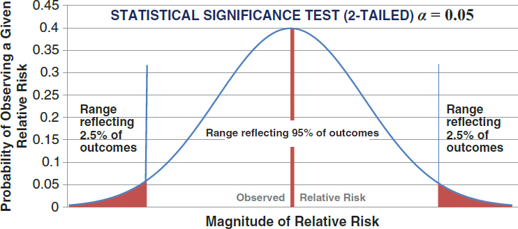
ranges in Figure 4. A significance test is ordinarily two-tailed, as depicted in Figure 4.113
There is some controversy among epidemiologists and biostatisticians about the appropriate role of significance testing.114 To the strictest significance testers,
113. Two-tailed p-values assume that the direction of the association, either greater or less than the null of 1.0, is not known, and thus distribute the probabilities on both sides of the null. For example, if a study estimated a relative risk of 4.0, a two-tailed p-value would include the probability that, if the null hypothesis is true, the study would find a relative risk either equal to or larger than 4.0 (the observed value) or equal to or less than 0.25 (the inverse of the observed value, i.e., 1/4.0). A one-tailed test, which is sometimes employed, considers only probabilities on the same side of the null as the study result. For a given alpha, a one-tailed test effectively doubles the probability of finding a significant effect in the hypothesized direction and is therefore controversial among epidemiologists and uncommon in epidemiologic studies. See In re Phenylpropanolamine (PPA) Prods. Liab. Litig., 289 F. Supp. 2d 1230, 1241 (W.D. Wash. 2003) (accepting the propriety of a one-tailed test for statistical significance in a toxic-substance case); United States v. Philip Morris USA, Inc., 449 F. Supp. 2d 1, 701 (D.D.C. 2006) (explaining the basis for EPA’s decision to use a one-tailed test in assessing whether secondhand smoke was a carcinogen). But see Good v. Fluor Daniel Corp., 222 F. Supp. 2d 1236, 1243 (E.D. Wash. 2002) (concluding that, in the circumstances presented, a one-tailed test on which the expert relied was not valid). For more on the difference between one-tailed and two-tailed tests, see Kaye & Stern, supra note 16.
114. In 2019, The American Statistician, a journal of the American Statistical Society, published an editorial that contained numerous “don’ts” in using statistical significance that many had previously violated. R. Wasserstein et al., Moving to a World Beyond p<0.05, 73 Am. Statistician 1 (Supp. 1, 2019). Some courts, contrary to the editorial’s prescriptions, have used statistically significant results as a threshold for acceptability of a study. The leading case advocating statistically significant studies is Brock v. Merrell Dow Pharms., Inc., 874 F.2d 307, 312 (5th Cir.), amended, 884 F.2d 167
any study whose p-value is greater than the level chosen for statistical significance should be rejected as inadequate to disprove the null hypothesis. However, the consensus among most epidemiologists is that conclusions about potential
(5th Cir. 1989). Overturning a jury verdict for the plaintiff in a Bendectin case, the court observed that no statistically significant study had been published that found an increased relative risk for birth defects in children whose mothers had taken Bendectin. A number of courts have followed the Brock decision or have indicated strong support for significance testing as a screening device. See, e.g., In re Zoloft (Sertraline Hydrochloride) Prod. Liab. Litig., 26 F. Supp. 3d 449, 456, 465 (E.D. Pa. 2014) (ruling that an expert witness’s reliance on non-statistically significant data was “not derived from principles and techniques of uncontroverted validity” and was a “departure from use of well-established epidemiological methods”); Wagoner v. Exxon Mobil Corp., 813 F. Supp. 2d 771, 800 (E.D. La. 2011) (“An opinion on general causation is inadmissible if it rests entirely on studies that do not show statistically significant results.”).
By contrast, a number of courts appear more cautious about using significance testing as a necessary condition, instead recognizing that assessing the likelihood of random error is important in determining the probative value of a study. In Allen, 588 F. Supp. at 417, the court stated, “The cold statement that a given relationship is not ‘statistically significant’ cannot be read to mean there is no probability of a relationship.” The Third Circuit described confidence intervals (i.e., the range of values that would be found in similar studies as a result of chance, with a specified level of confidence) and their use as an alternative to statistical significance in DeLuca v. Merrell Dow Pharms., Inc., 911 F.2d 941, 948–49 (3d Cir. 1990). See also, e.g., In re Lipitor (Atorvastatin Calcium) Mktg., Sales Pracs. & Prods. Liab. Litig., 892 F.3d 624, 642 (4th Cir. 2018) (“[W]e decline to establish a bright-line rule requiring experts to rely only on evidence that is statistically significant or else have their opinions excluded.”); Milward v. Acuity Specialty Prod. Grp., Inc., 639 F.3d 11, 24–25 (1st Cir. 2011) (“the district court read too much into the paucity of statistically significant epidemiological studies” since it would be “very difficult to perform an epidemiological study of the causes of [the disease] that would yield statistically significant results”).
In Daubert v. Merrell Dow Pharms., Inc., 509 U.S. 579 (1993), although the trial court had relied in part on the absence of statistically significant epidemiologic studies, the Supreme Court did not explicitly address the matter. One commentator concluded that “Daubert did not set a threshold level of statistical significance either for admissibility or for sufficiency of scientific evidence.” Developments in the Law, supra note 108, at 1535–36, 1540–46. The Supreme Court in General Electric Co., 522 U.S. at 145–47, adverted to the lack of statistical significance in one study relied on by an expert as a ground for ruling that the district court had not abused its discretion in excluding the expert’s testimony. In a different context—securities fraud—the Supreme Court held that a lack of statistical significance in adverse event reports did not disqualify them from being “material and requiring disclosure.” Matrixx Initiatives, Inc. v. Siracusano, 563 U.S. 27 (2011). In the course of its opinion, the Court explained:
A lack of statistically significant data does not mean that medical experts have no reliable basis for inferring a causal link between a drug and adverse events. As Matrixx itself concedes, medical experts rely on other evidence to establish an inference of causation. We note that courts frequently permit expert testimony on causation based on evidence other than statistical significance. We need not consider whether the expert testimony was properly admitted in those cases, and we do not attempt to define here what constitutes reliable evidence of causation. It suffices to note that, as these courts have recognized, “medical professionals and researchers do not limit the data they consider to the results of randomized clinical trials or to statistically significant evidence.” Matrixx, 563 U.S. at 40–41 (citations and footnote omitted).
associations should not rely on strict significance testing115 and that it is inappropriate either to reject all results that fail to meet the specified p-value or to accept all results that do meet this level.116 Epidemiologists have become increasingly sophisticated in addressing the issue of random error and examining the data from a study that may provide information about the relation between an agent and a disease, without the necessity of basing their conclusions solely on statistical significance.117 Meta-analysis, a method for pooling the results of multiple studies, sometimes can ameliorate concerns about random error present in a single study.118
Calculation of a confidence interval permits a more refined assessment of appropriate inferences about the association found in an epidemiologic study.119 A confidence interval represents a range of possible values calculated from the
115. In addition to criticism of significance testing, many lawyers, judges, and legal academics have incorrectly stated that using an alpha of 0.05 for statistical significance testing imposes a burden of proof on the plaintiff far higher than the civil burden of a preponderance of the evidence (i.e., greater than 50%). See Michael D. Green, Science Is to Law as the Burden of Proof Is to Significance Testing, 37 Jurimetrics J. 205, 221 n.67 (1997) (book review) (citing many examples).
To fully explain why this comparison is mistaken would require more space and detail than is feasible here. We sketch out a brief explanation. First, using an alpha of 0.50 would not be equivalent to saying that the probability that the association found is real is 50%, and the probability that it is a result of random error is 50%. Statistical methodology does not permit assessment of those probabilities. Second, significance testing only bears on whether the observed magnitude of association arose as a result of random chance, not on whether the null hypothesis is true. Third, using stringent significance testing to avoid false-positive error comes at a complementary cost of inducing false-negative error. Fourth, alpha does not address the likelihood that a plaintiff’s disease was caused by exposure to the agent; the magnitude of the association bears on that question. See section titled “Specific Causation” below. See Green, supra note 70, at 686–89; see also David H. Kaye, Apples and Oranges: Confidence Coefficients and the Burden of Persuasion, 73 Cornell L. Rev. 54, 66 (1987); Kaye & Stern, supra note 16, “Evaluating Hypothesis Tests”; Turpin v. Merrell Dow Pharms., Inc., 959 F.2d 1349, 1357 n.2 (6th Cir. 1992); cf. DeLuca v. Merrell Dow Pharms., Inc., 911 F.2d 941, 959 n.24 (3d Cir. 1990) (“The relationship between confidence levels and the more likely than not standard of proof is a very complex one . . . and in the absence of more education than can be found in this record, we decline to comment further on it.”).
116. For a hypercritical assessment of statistical significance testing by two economists that nevertheless identifies much inappropriate overreliance on it, see Stephen T. Ziliak & Deidre N. McCloskey, The Cult of Statistical Significance (2008).
117. See Sanders, supra note 16, at 342 (describing the improved handling and reporting of statistical analysis in studies of Bendectin after 1980).
118. See section titled “Methods for Synthesizing or Combining the Results of Multiple Studies” below.
119. Kenneth Rothman, Professor of Public Health at Boston University and Adjunct Professor of Epidemiology at the Harvard School of Public Health, is one of the leaders in advocating the use of confidence intervals and rejecting strict significance testing. See DeLuca v. Merrell Dow Pharms., Inc., 911 F.2d 941, 947 (3d Cir. 1990) (discussing Rothman’s views on the appropriate level of alpha and the use of confidence intervals); Turpin v. Merrell Dow Pharms., Inc., 959 F.2d 1349, 1353–54 n.1 (6th Cir. 1992) (discussing the relationship among confidence intervals, alpha, and statistical power). See also Cook v. Rockwell Int’l Corp., 580 F. Supp. 2d 1071, 1100–01 (D. Colo. 2006) (discussing confidence intervals, alpha, and significance testing). For a discussion of
results of a study. For example, a 95% confidence interval signifies that 95% of the confidence intervals generated by multiple identical studies would include the true value. The width of the interval reflects random error. The narrower the confidence interval, the more statistically stable the results of the study.
The advantage of a confidence interval is that it displays more information than significance testing. Statistically significant does not convey the magnitude of the association found in the study or reveal how statistically stable that association is. A confidence interval shows boundaries of the relative risk (or other measure of association) based on selected levels of alpha or statistical significance. Just as the p-value does not provide the probability that the risk estimate found in a study is correct, the confidence interval does not provide the range within which the true risk is likely to lie. In other words, it is a misconception to interpret a 95% confidence interval as representing an interval within which the true value has a 95% probability of being found. Though some types of statistical analyses (referred to as Bayesian statistics) can generate intervals with this interpretation (referred to as credible intervals), most published research does not.120 An example of two confidence intervals that might be calculated for a given relative risk is displayed in Figure 5.
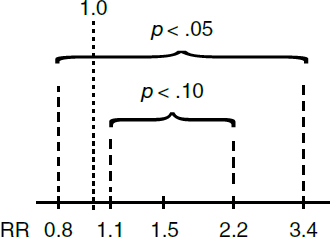
The confidence intervals shown in Figure 5 are for a hypothetical study that found a relative risk of 1.5, with boundaries of 0.8 to 3.4 when alpha is set to 0.05 (equivalently, a confidence level of 0.95), and with boundaries of 1.1 to 2.2 when alpha is set to 0.10 (equivalently, a confidence level of 0.90). The confidence interval for alpha equal to 0.10 is narrower because it encompasses only
the use of confidence intervals in evaluating sampling error more generally than in the epidemiologic context, see Kaye & Stern, supra note 16, “What Is the Confidence Interval?”
120. See Jonathan A.C. Sterne & George Davey Smith, Sifting the Evidence: What’s Wrong with Significance Tests, 322 BMJ 226, 228 (2001) (comparing frequentist significance testing with Bayesian statistical approaches).
90% of the expected intervals. By contrast, the confidence interval for alpha equal to 0.05 includes the expected outcomes for 95% of the intervals. To generalize this point, the lower the alpha chosen (and therefore the more stringent the exclusion of positive results as possible random error), the wider the confidence interval. At a given alpha, the width of the confidence interval is determined by sample size. All other things being equal, the larger the sample size, the narrower the confidence boundaries (indicating greater numerical stability or precision). For a given risk estimate, a narrower confidence interval reflects a decreased likelihood that an association found in a particular study would occur by chance if the true association is 1.0.121
For the example in Figure 5, the boundaries of the confidence interval with alpha set at 0.05 encompass a relative risk of 1.0, and the result would be said not to be statistically significant at the 0.05 level. Alternatively, if the confidence boundaries are defined as an alpha equal to 0.10, then the confidence interval no longer includes a relative risk of 1.0, and the result could be described as statistically significant at the 0.10 level. Common practice in epidemiologic studies is to estimate 95% confidence intervals.
False Negatives
As Figure 5 illustrates, false positives can be reduced by adopting more stringent values for alpha, which increases the likelihood that a result will fail the selected test of statistical significance. Using an alpha of 0.05 will result in fewer false positives than using an alpha of 0.10. An alpha of 0.01 or 0.001 would produce even fewer false positives.122 The tradeoff for reducing false positives is an increase in false-negative errors (also called beta errors or Type II errors123). This concept reflects the possibility that a study will be interpreted as negative (providing no grounds to reject the null hypothesis), when in fact there is a true
121. Where multiple epidemiologic studies are available, a technique known as meta-analysis may be used to combine the results of the studies (see section titled “Methods for Synthesizing or Combining the Results of Multiple Studies” below), thereby reducing the numerical instability of all the studies. See generally Diana B. Petitti, Meta-Analysis, Decision Analysis, and Cost-Effectiveness Analysis: Methods for Quantitative Synthesis in Medicine (2d ed. 2000).
122. As described above, supra note 109, in genome-wide association studies, which search the entire human genome to see if variations in genes are associated with variable disease risk, alpha is commonly set at 5 × 10⁻⁸, allowing one false positive per 20 million tests. Some researchers, worried that such stringent significance testing causes too many real associations to be rejected as potential chance results, have proposed ameliorative approaches. See Shrahyashi Biswas et al., A Framework for Pathway Knowledge Driven Prioritization in Genome-wide Association Studies, 44 Genetic Epidemiology 841 (2020), https://doi.org/10.1002/gepi.22345.
123. See A Dictionary of Epidemiology 99 (Miquel Porta et al. eds., 6th ed. 2014).
association of a specified magnitude.124 The probability of such an error, commonly called beta in statistical analyses, can be calculated for any study.
Statistical Power
When a study fails to find a statistically significant association, an important question is whether the result tends to exonerate the agent’s toxicity or is essentially inconclusive with regard to toxicity.125 The concept of statistical power can be helpful in evaluating whether a study’s results, if not statistically significant, are exonerative or inconclusive.126
The power of a study is the probability of finding a statistically significant association of a given magnitude (if it exists). The power of a study depends on several factors: the sample size; the level of alpha (or statistical significance) specified; the background incidence of disease; and the specified magnitude of the association (i.e., the size of the relative risk) that the researcher would like to detect.127 Power curves can be constructed that show the likelihood of finding
124. See also DeLuca v. Merrell Dow Pharms., Inc., 911 F.2d 941, 947 (3d Cir. 1990); In re Testosterone Replacement Therapy Prods. Liab. Litig. Coordinated Pretrial Proc., No. 14 C 1748, 2017 WL 1833173, at *12 n.12 (N.D. Ill. May 8, 2017) (concluding expert’s testimony comparing likelihood of Type I and Type II errors “will be helpful to the jury”).
125. Even when a study or body of studies tends to exonerate an agent, that does not establish that the agent is absolutely safe. See Cooley v. Lincoln Elec. Co., 693 F. Supp. 2d 767 (N.D. Ohio 2010). Epidemiology is not able to provide such evidence.
126. See Fienberg et al., supra note 101, at 22–23; Sander Greenland, Null Misinterpretation in Statistical Testing and Its Impact on Health Risk Assessment, 53 Preventative Med. 225 (2011), https://doi.org/10.1016/j.ypmed.2011.08.010 (explaining that statistical nonsignificance does not necessarily provide evidence for the null hypothesis and identifying such errors in reasoning). Thus, in Smith v. Wyeth-Ayerst Labs. Co., 278 F. Supp. 2d 684, 693 (W.D.N.C. 2003) and Cooley v. Lincoln Elec. Co., 693 F. Supp. 2d 767, 773 (N.D. Ohio 2010), the courts recognized that the power of a study was critical to assessing whether the failure of the study to find a statistically significant association was exonerative of the agent or inconclusive. See also Procter & Gamble Pharms., Inc. v. Hoffmann-LaRoche Inc., No. 06 CIV. 0034 (PAC), 2006 WL 2588002, at *32 n.16 (S.D.N.Y. Sept. 6, 2006) (discussing power curves and quoting the second edition of this reference guide); In re Phenylpropanolamine (PPA) Prods. Liab. Litig., 289 F. Supp. 2d 1230, 1243–44 (W.D. Wash. 2003) (explaining expert’s testimony that “statistical reassurance as to lack of an effect would require an upper bound of a reasonable confidence interval close to the null value”); Ruff v. EnsignBickford Indus., Inc., 168 F. Supp. 2d 1271, 1281 (D. Utah 2001) (explaining why study should be treated as inconclusive rather than exonerative based on small number of subjects in the study).
127. See Malcolm Gladwell, How Safe Are Your Breasts?, New Republic, Oct. 24, 1994, at 22, 26, https://perma.cc/83AP-4AGM; Kenneth J. Rothman & Timothy L. Lash, Precision and Study Size, in Lash et al., supra note 50, at 333, 354–55. For continuous health outcomes such as child IQ, the magnitude of the association is measured differently (see supra text accompanying footnotes 75-76 and infra entry “beta coefficient” in the Glossary of Terms), and instead of background incidence the statistical power would depend in part on the background variability of the outcome.
any given relative risk in light of these factors. Often, power curves are used in the design of a study to determine what size a study population should be.128
The power of a study is the complement of beta (1−β). Thus, a study with a likelihood of 0.25 of failing to detect a true relative risk of 2.0129 or greater has a power of 0.75. This means the study has a 75% chance of detecting a true relative risk of 2.0. If the power of a null study to find a relative risk of 2.0 or greater is low, it has substantially less probative value than a study with similar results but a higher power.130
Choosing the sample size is the main way in which a researcher can affect the power of the study. Because studies with larger sample sizes are more powerful than studies with smaller sample sizes (everything else being equal), a null study with a large sample size is given more credence than a similar null study with a smaller sample size.131
Biases
Other than sampling error, another reason an epidemiologic study might find an invalid or inaccurate association is systematic error or bias, as distinguished from random error. Bias may arise in the design or conduct of a study, data collection, or data analysis. Some biases (such as confounding, described below) may also be inherent to the natural relation between the agent of interest and the disease under study.
The meaning of scientific bias differs from conventional (and legal) usage, in which bias refers to a partisan point of view.132 When scientists use the term bias, they refer to anything that results in a systematic (nonrandom) error in a study result and thereby compromises the study’s validity. The statistical measures that address possible sampling error—significance tests, confidence intervals, and power—do not address systematic error (bias), because bias does not result from random chance in the selection of study subjects.133
128. For examples of power curves, see Kenneth J. Rothman, Modern Epidemiology 80 (1986); Pagano & Gauvreau, supra note 86, at 239. For a different graphical presentation showing how a smaller study size results in a wider 95% confidence interval for a given level of absolute and relative risk, see Rothman & Lash, supra note 127, at 360.
129. We use a relative risk of 2.0 for illustrative purposes because of the legal significance courts have attributed to this magnitude of association. See section titled “Specific Causation” below.
130. See also Kaye & Stern, supra note 16; section titled “Effect Modification” below.
131. See id. for a more detailed discussion of statistical power.
132. See A Dictionary of Epidemiology, supra note 123, at 21; Edmond A. Murphy, The Logic of Medicine 239–62 (1976).
133. See Green, supra note 70, at 667–68; Vincent M. Brannigan et al., Risk, Statistical Inference, and the Law of Evidence: The Use of Epidemiological Data in Toxic Tort Cases, 12 Risk Analysis 343, 344–45 (1992), https://doi.org/10.1111/j.1539-6924.1992.tb00686.x. Contrary to the statement in
Most epidemiologic studies have some degree of bias that may affect the outcome. If major bias is present, it may invalidate the study results. Identifying biases, however, can be challenging and requires expertise in both epidemiologic methods as well as the subject matter at hand. In reviewing the validity of an epidemiologic study, the epidemiologist should identify potential biases and analyze the amount or kind of error that might have been induced by the bias. In some cases, the potential direction of the bias can be determined and, depending on the specific type of bias, it may exaggerate the real association, dilute it, completely mask it, or even reverse its direction.
Biases are generally classified in three categories: selection bias, information bias, and confounding bias. Selection bias can result from differences between individuals selected for a study and the larger population about which researchers want to make inferences based on the study results. Information bias can arise from errors in measuring exposure, disease, or other relevant variables. Confounding bias can occur if other causal factors influence the association between exposure to an agent and a disease.
Selection Bias
Selection bias refers to the error in an observed association that results from the method of selection of study participants, such as cases and controls (in a case-control study) or exposed and unexposed individuals (in a cohort study). Selection bias can occur in several ways. One common source of selection bias is the existence of non-random differences between individuals who are selected as study participants and those who are not.134
The selection of an appropriate control group has been described as the Achilles’ heel of a case-control study.135 Controls should be drawn from the same
at least one early toxic tort case, see, e.g., Brock v. Merrell Dow Pharms., Inc., 874 F.2d 307, 312 (5th Cir. 1989), a study’s use of confidence intervals cannot “incorporate the possibility” of bias in the data. A statistically significant result with a narrow 95% confidence interval could be incorrect if bias exists. See In re Zoloft (Sertraline Hydrochloride) Prods. Liab. Litig., 858 F.3d 787, 793 (3d Cir. 2017) (“If a causal connection does not actually exist, significant findings can still occur due to, inter alia, inability to control for a confounding effect or detection bias.”).
134. In In re “Agent Orange” Prod. Liab. Litig., 597 F. Supp. 740, 783 (E.D.N.Y. 1985), aff’d, 818 F.2d 145 (2d Cir. 1987), the court expressed concern about selection bias. The exposed cohort consisted of young, healthy men who served in Vietnam. Comparing the mortality rate of the exposed cohort and that of a control group made up of civilians might have resulted in error that was a result of selection bias. Failing to account for health status as an independent variable tends to understate any association between exposure and disease in studies in which the exposed cohort is healthier. See also In re Baycol Prods. Litig., 532 F. Supp. 2d 1029, 1043 (D. Minn. 2007) (upholding admissibility of testimony by expert witness who criticized study based on selection bias).
135. William B. Kannel & Thomas R. Dawber, Coffee and Coronary Disease, 289 NEJM 100 (1973) (editorial), https://doi/full/10.1056/NEJM197410242911703.
source population (a concept often referred to as the study base) that produced the cases. Doing so avoids the possibility that the controls will have different risk factors for the disease than the cases. Selecting control participants becomes problematic if the control participants are selected for reasons that are related to their exposure (or lack thereof) to the agent being studied. For example, a study of the effect of smoking on heart disease will suffer selection bias if subjects of the study are volunteers and the decision to volunteer is affected by both being a smoker (perhaps smokers are more likely to choose to participate in a study due to concerns about their health) and having a family history of heart disease (which increases the probability that they will suffer from the disease due to genetics). In this case, the association will be biased upward because smokers with higher probabilities of heart disease will be more likely to self-select for the study.
Hospital-based studies, which are relatively common among researchers located in medical centers, illustrate the problem. Suppose an association is found between coffee drinking and coronary heart disease in a study using hospital patients as controls. The problem is that the hospitalized control group may include individuals who had been advised against drinking coffee for medical reasons, such as to prevent the aggravation of a peptic ulcer. In other words, the controls may become eligible for the study because of their medical condition, which is in turn related to their exposure status—their likelihood of avoiding coffee. If this is true, the amount of coffee drinking in the control group would understate the extent of coffee drinking expected in people who do not have the disease and thus would bias upwardly (i.e., exaggerate) any odds ratio observed.136 Bias in hospital studies may also understate the true odds ratio when the exposures at issue increase the likelihood of cases being hospitalized and also contribute to the controls’ chances of hospitalization.
Just as cases and controls in case-control studies should be selected independently of their exposure status, the exposed and unexposed participants in cohort studies should be selected independently of their disease risk.137 For example, if women with hysterectomies are overrepresented among exposed (smoking) women in a cohort study of the connection between smoking and cervical
136. Hershel Jick et al., Coffee and Myocardial Infarction, 289 NEJM 63 (1973), https://doi.org/10.1056/NEJM197307122890203 (finding an association between coffee drinking and coronary heart disease using hospital patients for controls).
137. Selection bias can introduce confounding factors (see section titled “Effect Modification” below) when unexposed controls may differ from the exposed cohort because exposure is associated with other risk (or protective) factors. Investigators can attempt to measure and adjust for those differences, as explained in the section titled “Effect Modification” below. See also Martha J. Radford & JoAnne M. Foody, How Do Observational Studies Expand the Evidence Base for Therapy?, 286 JAMA 1228 (2001), https://doi.org/10.1001/jama.286.10.1228 (discussing the use of propensity analysis to adjust for potential confounding and selection biases that may occur from nonrandomization in observational epidemiology).
cancer, this could understate the association between the exposure and the disease. This is so because women who have a hysterectomy cannot develop cervical cancer so the overrepresentation of women with hysterectomies would reduce the number of smoking women who develop cervical cancer in the study. If exposure to the agent is also related to participation in the study, selection bias could occur. For example, if women who are more health-conscious (and therefore are less likely to smoke) were also more likely to enroll in the study, a spurious association would be created between smoking and cervical cancer.
A further source of selection bias occurs when those selected to participate decline to participate or drop out before the study is completed. Many studies have shown that individuals who choose to participate or remain in studies over time differ substantially from those who do not. If a substantial portion of individuals declines to participate, the researcher should investigate whether those who declined are different from those who agreed. If data are available on nonparticipants, the researcher can compare relevant characteristics of those who participate with those who do not, to show the extent to which the two groups are comparable. Similarly, if a significant number of subjects drop out of a study before completion, the remaining subjects may not be representative of the original study populations. The researcher should examine whether that is the case.
The fact that a study may suffer from selection bias does not necessarily invalidate its results. A number of factors may suggest that a bias, if present, had only a limited effect. If the association is particularly strong, for example, bias is less likely to account for all of it. In addition, a consistent association across different control groups suggests that possible biases applicable to a particular control group are not invalidating. Similarly, a dose–response relationship (see section titled “Dose–Response Relationship” below) found among multiple groups exposed to different doses of the agent may provide additional evidence that biases applicable to the exposed group are not a major problem. However, the converse may not necessarily be true as the risk of disease associated with some agents may not consistently increase with exposure level, a concept referred to as nonlinearity.138 Finally, it is important to note that if data are available about nonparticipants or those lost to follow-up, statistical methods can be applied to mitigate selection bias.
Information Bias
Information bias is a result of inaccurate information primarily about either the disease or the exposure status of the study participants.139 In assessing whether the data may reflect inaccurate information, one must assess whether the data
138. See infra notes 237–41 and accompanying text.
139. Incorrect information about potential confounders can also bias the results of a study.
were collected from objective and reliable sources. Medical records, government documents, employment records, death certificates, and interviews are examples of data sources that are used by epidemiologists to measure either exposure or disease status. The accuracy of a particular source may affect the validity of a research finding. For example, using employment records to gather information about exposure to narcotics probably would lead to inaccurate results, because employees tend to keep such information private. If the researcher uses an unreliable source of data, the study may not be useful.
The kinds of quality-control procedures used may affect the accuracy of the data. For data collected by interview, quality-control procedures should probe the reliability of the individual and whether the information is verified by other sources whenever possible. For data collected and analyzed in the laboratory, quality-control procedures should assess the validity and reliability of the laboratory tests.
Exposure information bias
Though information bias may affect the results of a study of any study design, this category of bias (exposure information bias) is an important consideration for retrospective studies, such as case-control studies, where researchers depend on information from the past to determine exposure.140 In some situations, the researcher may be required to interview the subjects to determine past exposures, thus relying on the subjects’ memories. Research has shown that individuals with disease (cases) tend to recall past exposures more readily than individuals with no disease (controls);141 this creates a potential for a type of information bias called recall bias.
For example, consider a case-control study conducted to examine the cause of congenital malformations. The epidemiologist is interested in whether the malformations were caused by an infection during the mother’s pregnancy. A group of mothers of infants with malformations (cases) and a group of mothers of infants with no malformation (controls) are interviewed regarding infections
140. Information bias can be a problem in cohort studies as well. When exposure is determined retrospectively, there can be a variety of impediments to obtaining accurate information. Similarly, when disease status is determined retrospectively, bias is a concern. The determination that asbestos is a cause of mesothelioma was hampered by inaccurate death certificates that identified lung cancer rather than mesothelioma, a rare form of cancer, as the cause of death. See I.J. Selikoff et al., Mortality Experience of Insulation Workers in the United States and Canada, 220 Annals N.Y. Acad. Sci. 91, 110–11 (1979), https://doi.org/10.1111/j.1749-6632.1979.tb18711.x; David E. Lilienfeld & Paul D. Gunderson, The “Missing Cases” of Pleural Malignant Mesothelioma in Minnesota, 1979–81: Preliminary Report, 101 Pub. Health Rep. 395, 397–98 (1986).
141. Steven S. Coughlin, Recall Bias in Epidemiological Studies, 43 J. Clinical Epidemiology 87 (1990).
during pregnancy. Mothers of children with malformations may recall an inconsequential fever or runny nose during pregnancy that readily would be forgotten by a mother who had a normal infant.142 Even if in reality the infection rate in mothers of children with malformations is no different from the rate in mothers of normal children, the result in this study would be an apparently higher rate of infection in the mothers of the children with the malformations solely on the basis of recall differences between the two groups.143
The issue of recall bias can sometimes be addressed by finding a second source of data to validate the subject’s response (e.g., blood-test results from prenatal visits or medical records that document symptoms of infection).144 Alternatively, the mothers’ responses to questions about other exposures that were not
142. Recall bias among parents whose babies had birth defects was a prominent issue in Bendectin cases. See, e.g., Brock, 874 F.2d at 311–12 (discussing recall bias among women who bear children with birth defects); Lynch v. Merrell-National Labs., 830 F.2d 1190, 1195 (1st Cir. 1987) (discussing a study’s attempt to “wash out ‘maternal-recall bias’”).
143. In a case similar to this hypothetical, Newman v. Motorola, Inc., 218 F. Supp. 2d 769, 778 (D. Md. 2002), the court considered a study of the effect of cell phone use on brain cancer and concluded that there was good reason to suspect that recall bias affected the results of the study, which found an association between cell phone use and cancers on the side of the head where the cell phone was used but no association between cell phone use and overall brain tumors. The court excluded plaintiff’s proposed expert testimony on causation. Id. at 783.
144. Two researchers who used a case-control study to examine the association between congenital heart disease and the mother’s use of drugs during pregnancy corroborated interview data with the mother’s medical records. See Sally Zierler & Kenneth J. Rothman, Congenital Heart Disease in Relation to Maternal Use of Bendectin and Other Drugs in Early Pregnancy, 313 NEJM 347, 347–48 (1985). Courts have considered researchers’ varied efforts to determine the extent to which recall bias affected study results. For example, in one case plaintiffs’ experts “pointed to studies that sought to validate self-reports of pesticide exposure and that found similar recall accuracy between cases and controls.” In re Roundup Prods. Liab. Litig., 390 F. Supp. 3d 1102, 1121 (N.D. Cal. 2018). In multidistrict litigation alleging that prolonged perineal use of talcum powder products caused ovarian cancer, an expert witness for plaintiffs acknowledged the possibility that recall bias affected the results of case-control studies, but opined that the possibility could be discounted because similar results were found in data collected both before and after widespread media coverage of the purported causal link. In re Johnson & Johnson Talcum Powder Mktg., Sales Pracs., & Prods. Litig., 509 F. Supp. 3d 116, 167 (D.N.J. 2020). The court concluded that “Defendants and their experts may disagree with Plaintiffs’ general causation experts’ assessment of recall bias in the case-control studies, but that does not render their opinions unreliable under Daubert.” Id. at 168. In another talcum powder case, plaintiffs relied on a case-control study in which the researchers lacked an independent source of data on the study subjects’ talcum powder use. But the researchers relied on a study of a different exposure, “in which retrospective recall could be compared to verifiable prospective data,” to provide a surrogate baseline measurement of inaccurate recall. Carl v. Johnson & Johnson, 237 A.3d 308, 327 (N.J. Super. Ct. App. Div. 2020). The researchers performed a sensitivity analysis that showed that even if their study suffered from twice as much recall bias, their result would still be statistically significant. Id. The court reversed the trial judge’s exclusion of plaintiffs’ expert testimony. Id. at 344.
expected to cause the disease may shed light on whether bias affected the recall of the relevant exposures.145
Bias may also result from reliance on interviews with surrogates who are individuals other than the study subjects. This is often necessary when, for example, a subject (in a case-control study) has died of the disease under investigation or may be too ill to be interviewed.
The quality of a study’s assessment of participants’ exposure can affect the credibility of an association with a health outcome.146 The extent of exposure147 can be obtained from a number of different sources, each of which has limitations and strengths.148
For estimating past exposures, epidemiologists often use indirect measures of exposure, such as interviewing workers and reviewing employment records. For
145. Analogously, an expert testified that because recall bias would be expected to affect reported exposures for people with any type of cancer, concerns about recall bias were diminished where “epidemiology studies on the whole observed associations only between” exposure to an herbicide and a particular type of cancer, rather than with “the other cancers about which participants were asked.” In re Roundup Prods. Liab. Litig., 390 F. Supp. 3d 1102, 1121 (N.D. Cal. 2018). The court concluded that “concerns about recall bias in these studies do not demand that a reliable expert opinion meaningfully discount the body of case-control studies when assessing causation.” Id.
146. The quality of exposure assessment in an epidemiologic study should be distinguished from the issue of the quality of the evidence of the extent of the plaintiff’s exposure, an issue that often arises in environmental-exposure cases. See infra note 150.
147. The exposure “dose” is defined in various ways, but dose often refers to the intensity or magnitude of exposure multiplied by the time exposed. See Bernard D. Goldstein, Toxic Torts: The Devil Is in the Dose, 15 J.L. & Pol’y 551, 554 (2008) (“Dose is defined as concentration multiplied by frequency or duration–it is not just the exposure level at any one point in time.”). Other definitions of dose may be more appropriate in light of the biological mechanism of the disease. See Emily White et al., Principles of Exposure Measurement in Epidemiology: Collecting, Evaluating, and Improving Measures of Disease Risk Factors (2d ed. 2008); National Research Council, Exposure Science in the 21st Century (2012). See also Gates v. Rohm & Haas Co., 655 F.3d 255, 260 (3d Cir. 2011) (affirming district court decision that an expert report that assumed a constant and average value of air pollutant exposure during lengthy time periods, which is considered “overly simplistic,” was insufficient evidence to establish dose). For a discussion of the difficulties of determining dose from atomic fallout, see Allen, 588 F. Supp. 247, 425–26, rev’d on other grounds, 816 F.2d 1417 (10th Cir. 1987).
The timing of exposure in relation to the life course may also be critical, especially if the disease of interest is a birth defect. In Smith v. Ortho Pharm. Corp., 770 F. Supp. 1561, 1577 (N.D. Ga. 1991), the court criticized a study for its inadequate measure of exposure to spermicides. The researchers had defined exposure as receipt of a prescription for spermicide within 600 days of delivery, but this definition of exposure is too broad because environmental agents are likely to cause birth defects only during a narrow band of time.
148. See In re Paoli R.R. Yard PCB Litig., No. 86-2229, 1992 U.S. Dist. LEXIS 18430, at *9–*11 (E.D. Pa. Oct. 21, 1992) (discussing valid methods of determining exposure to chemicals). Exposure science is a discipline that assesses exposure and its extent and is addressed in another reference guide in this manual. See M. Elizabeth Marder & Joseph V. Rodricks, Reference Guide on Exposure Science and Exposure Assessment, “Understanding Human Exposure: Key Concepts,” in this manual.
example, a study might treat all those employed to install asbestos insulation as having been exposed to asbestos during the period that they were so employed. However, there may be a wide variation of exposure within any job, and therefore this job-classification measure may not accurately determine individual levels of exposure.149 If the agent of interest is a drug, medical or hospital records often can be used to determine past exposure. Retrospective studies that determine past exposures indirectly are usually less accurate than prospective studies or follow-up studies, including ones in which a drug or medical intervention is the agent of interest.
Exposure to the agent can also be measured directly. To directly determine an individual’s level, duration, and timing of exposure to an agent, researchers can use biological markers, or biomarkers, when they are available.150 A biomarker
149. Occupational epidemiologists frequently employ study designs that consider all agents to which workers in a particular occupation are exposed because they seek to determine the hazards associated with that occupation. Isolating one of the agents for examination would be difficult if not impossible. These studies, then, present difficulties when used in court in support of a claim by a plaintiff who was exposed to only one or some of the agents that were present at the worksite that was the subject of the study. See, e.g., Knight v. Kirby Inland Marine Inc., 482 F.3d 347, 352–53 (5th Cir. 2007) (concluding that case-control studies of cancer that entailed exposure to a variety of organic solvents at job sites did not support claims of plaintiffs who claimed exposure to benzene caused their cancers).
150. A different, but related, problem often arises in court. Determining the plaintiff’s exposure to the alleged toxic substance always involves a retrospective determination and may involve difficulties similar to those faced by an epidemiologist planning a study. Thus, in John’s Heating Serv. v. Lamb, 46 P.3d 1024 (Alaska 2002), plaintiffs were exposed to carbon monoxide because of defendants’ negligence with respect to a home furnace. The court observed: “[W]hile precise information concerning the exposure necessary to cause specific harm to humans and exact details pertaining to the plaintiff’s exposure are beneficial, such evidence is not always available, or necessary, to demonstrate that a substance is toxic to humans given substantial exposure and need not invariably provide the basis for an expert’s opinion on causation.” Id. at 1035 (quoting Westberry v. Gislaved Gummi AB, 178 F.3d 257, 264 (4th Cir. 1999)). See generally Restatement (Third) of Torts: Liability for Physical and Emotional Harm § 28 cmt. c(2) & rptrs. note (2010).
Even if a biomarker exists for exposure to a particular agent, it may be problematic to attempt to use that biomarker as a measure of a plaintiff’s past exposure to that agent. As described in the next paragraph, the persistence of biomarkers in the body following an exposure varies. Because of the long latency period between exposure and the manifestation of disease that is characteristic of many toxic tort cases, biomarker measurements that are available at the time of litigation may not accurately reflect a plaintiff’s much earlier exposure to a toxicant.
To address the problem of determining a plaintiff’s exposure in asbestos cases, a number of courts have adopted a requirement that the plaintiff demonstrate (1) regular use by an employer of the defendant’s asbestos-containing product; (2) the plaintiff’s proximity to that product; and (3) exposure over an extended period of time. See, e.g., Lohrmann v. Pittsburgh Corning Corp., 782 F.2d 1156, 1162–64 (4th Cir. 1986); Gregg v. V-J Auto Parts, Inc., 943 A.2d 216, 226 (Pa. 2007); see also James v. Bessemer Processing Co., 714 A.2d 898, 911–14 (N.J. 1998) (applying same standard to a claim involving substances other than asbestos and holding that plaintiff presented sufficient evidence of exposure to certain substances in particular manufacturers’ products to withstand summary judgment). Other courts have imposed more stringent requirements. E.g., Bostic v. Georgia-Pacific Corp., 439 S.W.3d 332, 353 (Tex. 2014) (holding that “the dose must be quantified but need not be established with mathematical precision,” although “the plaintiff must prove with
may be the actual parent compound to which an individual is exposed, a metabolite of the parent compound, or some other measure that reflects an exposure-induced alteration in biologic systems at the functional or molecular level.151 Measurements can be made in various biologic materials, including blood, urine, amniotic fluid, breast milk, seminal fluid, fecal material, hair, and nails. The appropriate matrix for measuring exposure is determined by the chemical agent and its properties.
Measurements in bodily fluids of chemicals with long half-lives (in the order of years), such as lead or DDT, are more likely to reflect exposure preceding a health outcome.152 Other chemical agents have short half-lives in the human body (e.g., bisphenol A, phenols), and thus the level of exposure indicated by a biomarker may not accurately reflect exposure during a critical window but may only reflect a very recent exposure (e.g., the last meal).153 Appropriate biological markers, however, are available only for a small number of toxicants.154
scientifically reliable expert testimony that the plaintiff’s exposure to the defendant’s product more than doubled the plaintiff’s risk of contracting the disease”). For criticism of Bostic’s requirement of a risk-doubling dose from each defendant’s product, see Steve C. Gold, Drywall Mud and Muddy Doctrine: How Not to Decide a Multiple-Exposure Mesothelioma Case, 49 Ind. L. Rev. 117 (2015).
151. Courts occasionally have noted the use of biomarkers to classify study subjects’ exposure levels. See, e.g., Nat’l Bank of Commerce (of El Dorado, Ark.) v. Dow Chem. Co., 965 F. Supp. 1490, 1553–54 (E.D. Ark. 1996) (favorably citing defendant’s expert’s testimony that praised a study in which low levels of cholinesterase in blood were used as a biomarker for exposure to cholinesterase-inhibiting pesticides). More often, courts must resolve disputes about whether a particular plaintiff displays a putative biomarker of exposure and the significance of the putative biomarker’s presence or absence. See, e.g., In re TMI Litig., 193 F.3d 613, 690–93 (3d Cir. 1999) (affirming exclusion of expert’s estimates of radiation doses plaintiffs received during nuclear accident fifteen years earlier because another methodology would provide more accurate estimates after such a long lapse of time); In re Flint Water Cases, 2021 WL 5356295, at *3 (E.D. Mich. Nov. 17, 2021) (denying motion to exclude testimony of plaintiff’s expert that measurement of lead levels in bone, rather than in blood, provided more accurate exposure assessment); Barlow v. Gen. Motors Corp., 595 F. Supp. 2d 929, 944 n.6 (S.D. Ind. 2009) (rejecting plaintiffs’ suggestion that body fat measurements would provide better marker of PCB exposure than blood measurements, where plaintiffs failed to produce evidence to that effect); Young v. Burton, 567 F. Supp. 2d 121, 136 (D.D.C. 2008) (excluding plaintiff’s expert testimony that certain biomarkers indicated exposure to mold five years earlier, where defense experts testified that the markers’ response to exposure lasts only minutes or hours).
152. If such a biomarker exists, retrospective studies may be able accurately to capture the exposure during critical biological windows depending on the half-life of the chemical and the time since that window.
153. In cases where the exposure has a short half-life, multiple measurements may be needed to accurately assess the level of exposure, unless they are reflective of typical exposure or if a single exposure can have a biologic effect. To use a biomarker to obtain an accurate assessment of exposure to such an agent, it may be necessary to measure the biomarker at multiple times, unless it is shown that a single measurement is representative of a longer-term exposure or that a single exposure could cause the health outcome at issue.
154. See Jessie P. Buckley et al., Exposure to Contemporary and Emerging Chemicals in Commerce Among Pregnant Women in the United States: The Environmental Influences on Child Health Outcome
In addition to biomarkers, epidemiologists may use measurements of non-biologic matrices such as water, dust, and air to assess exposure to agents found in those media.155 Sometimes monitoring devices can be used to measure such environmental exposures directly, but monitoring data often are not available for exposures that have occurred in the past unless they are routinely collected, such as through governmental air or water monitoring.
The route (e.g., inhalation or absorption), duration, and intensity of exposure also are important factors. Even with environmental monitoring, the dose measured in the environment generally is not the same as the dose that reaches internal target organs. If the researcher has calculated the internal dose of exposure, the scientific basis for this calculation should be examined for soundness.156
Disease information bias
Information bias may also result from inaccurate measurement of disease status. The quality and sophistication of the diagnostic methods used to detect a disease should be assessed.157 The proportion of subjects eligible for study who were
(ECHO) Program, 56 Env’t Sci. & Tech. 6560, 6560 (2022), https://doi.org/10.1021/acs.est.1c08942 (National Health and Nutrition Examination Survey (NHANES) provides data on exposure to 350 chemicals, a small fraction of the number of chemicals in use); Angela N.H. Creager, Human Bodies as Chemical Sensors: A History of Biomonitoring for Environmental Health and Regulation, 70 Studs. Hist. & Phil. Sci. 70, 76 (2018), https://doi.org/10.1016/j.shpsa.2018.05.010 (“For the past quarter century, research on biomarkers and genetic dosimetry has seemed poised to change environmental public health by offering more sensitive tools for measuring chemical exposure. Yet so far these tools have not displaced the widespread reliance on methods of chemical analysis.”); Steve C. Gold, The More We Know, The Less Intelligent We Are?—How Genomic Information Should, And Should Not, Change Toxic Tort Causation Doctrine, 34 Harv. Env’t L. Rev. 370 (2010) (describing circumstances where courts can improve their ability to link toxic substances to human illness by properly understanding and utilizing genomic information and analyzing biomarkers); Gary E. Marchant, Genetic Data in Toxic Tort Litigation, 14 J. L. & Pol’y 7, 18–32 (2006) (explaining concept of biomarkers and how they might be used to provide evidence of: (1) exposure or dose, (2) general and specific causation, and (3) identifying those with greater risks of future disease; discussing cases in which biomarkers were employed; and concluding, “genomic data [like biomarkers] have enormous potential to make toxic tort litigation more informed, consistent and fair”).
155. For example, concentrations of perflouorooctanoic acid (PFOA, a so-called “forever chemical”) found in a drinking water supply, levels of lead in dust in a home, or levels of polycyclic aromatic hydrocarbons (PAHs) or fine particulate matter (PM2.5) in the ambient air may be used to estimate exposures of the people who drink the water, live in the home, or breathe the air.
156. See also Eaton et al., supra note 60.
157. The hazards of adversarial review of epidemiologic studies to determine bias are highlighted by O’Neill v. Novartis Consumer Health, Inc., 55 Cal. Rptr. 3d 551, 558–60 (Ct. App. 2007). Defendant’s experts criticized a case-control study relied on by plaintiff on the ground that there was misclassification of exposure status among the cases. Plaintiff objected to this criticism because defendant’s experts had only examined the cases for exposure misclassification, which would tend
actually examined should be determined. If, for example, many of the subjects refused to be tested, the fact that the test used was of high quality may be of relatively little value given the potential for selection bias.
The scientific validity of the research findings is influenced by the accuracy of the diagnosis of disease or health status under study.158 The disease must be one that is recognized and defined to enable accurate diagnoses. To ensure that the diagnoses of study subjects are in fact accurate, diagnostic criteria accepted by the medical community should be used.159 For example, a researcher
to exaggerate any association by providing an inaccurately inflated measure of exposure in the cases. The experts failed to examine whether there was misclassification in the controls, which, if it existed, would tend to incorrectly diminish any association.
158. In In re Swine Flu Immunization Prods. Liab. Litig., 508 F. Supp. 897, 903 (D. Colo. 1981), aff’d sub nom. Lima v. United States, 708 F.2d 502 (10th Cir. 1983), the court critically evaluated a study relied on by an expert whose testimony was stricken. In that study, determination of whether a patient had Guillain-Barré syndrome was made by medical clerks, not physicians who were familiar with diagnostic criteria.
159. See generally Robert H. Friis & Thomas A. Sellers, Epidemiology for Public Health Practice 494 (6th ed. 2021) (in a case-control study, “the definition of a case is influenced by a number of factors, including whether there are standard diagnostic criteria . . . and whether the criteria to diagnose the disease are subjective or objective”).
Classification problems have affected the study of agent–disease links that later became the subject of litigation, for example the under-reporting of deaths due to mesothelioma. See supra note 140. Few court opinions, however, have addressed misclassification bias as the basis of a challenge to the validity of epidemiologic studies. See, e.g., In re Lipitor (Atorvastatin Calcium) Mktg., Sales Pracs., & Prods. Liab. Litig. (No. II) MDL 2502, 892 F.3d 624, 635–38 (4th Cir. 2018) (affirming exclusion of expert testimony where expert based opinion on reanalysis of epidemiologic study data using a different disease definition); Rochkind v. Stevenson, 164 A.3d 254, 261–62 (Md. 2017) (reversing admission of expert testimony opining that exposure to lead can cause attention deficit-hyperactivity disorder (ADHD) where expert relied on epidemiologic studies showing association with attention decrements in general but not with ADHD as defined by diagnostic criteria); In re Lipitor (Atorvastatin Calcium) Mktg., Sales Pracs., & Prods. Liab. Litig., 174 F. Supp. 3d 911, 917 n.5 (D.S.C. 2016) (noting that where one study found a statistically significant association, but another did not, the difference could be explained by the latter study’s use of a more restrictive disease definition but making “no value judgments” with respect to either study’s quality).
A related but subtly different issue arises more frequently: disputes about whether a plaintiff has been diagnosed accurately with a disease that has been (or could be) the subject of epidemiologic study. See, e.g., Grant v. Bristol-Myers Squibb, 97 F. Supp. 2d 986, 992 (D. Ariz. 2000) (“where experts propose that breast implants cause a disease but cannot specify the criteria for diagnosing the disease, it is incapable of epidemiologic testing[, rendering] the experts’ methods insufficiently reliable to help the jury”); Burton v. Wyeth-Ayerst Labs., 513 F. Supp. 2d 719, 722–24 (N.D. Tex. 2007) (parties disputed whether cardiology problem involved two separate diseases or only one; court concluded that all experts in the case reflected a view that there was but a single disease); Nat’l Bank of Commerce (of El Dorado, Ark.) v. Dow Chem. Co., 965 F. Supp. 1490 (E.D. Ark. 1996) (where children exposed in utero to pesticides suffered from birth defects, parties disputed whether children’s symptoms supported diagnosis of inherited syndromes); In re Breast Implant Cases, 942 F. Supp. 958, 961 (E.D.N.Y. & S.D.N.Y. 1996) (rejecting plaintiffs’ experts’ testimony that breast implants caused a “new undifferentiated atypical disease” with “hundreds of symptoms”).
interested in studying spontaneous abortion in the first trimester must determine that study subjects are pregnant. If that determination were made based on the results of home pregnancy tests at a time when home pregnancy tests were known to have a high rate of false-positive results (indicating pregnancy when the woman is not pregnant), the study will overestimate the number of spontaneous abortions.
Information bias due to misclassification
Misclassification is a consequence of information bias in which, because of problems with the information available, individuals in the study may be misclassified as to exposure status or disease status. Bias due to exposure misclassification can be differential or nondifferential. In nondifferential misclassification (also called random misclassification), the inaccuracies in determining exposure are independent of disease status, or the inaccuracies in diagnoses are independent of exposure status—in other words, the data are crude and contain some level of random error. This is a common problem.
Generally, nondifferential misclassification shifts the study’s result toward a finding of no effect.160 Thus, if errors are nondifferential, an apparent association between an exposure and disease would not be a product of incorrect classification. Instead, nondifferential misclassification generally underestimates the true size of the association. Studies that find no association and are likely affected by a fair amount of nondifferential misclassification should therefore be regarded with suspicion. In fact, it has been shown that under some conditions, severe nondifferential misclassification could result in an association that suggests that an agent reduces the risk of disease, when in fact exposure to the agent increases the risk. However, it is important to note that nondifferential misclassification on its own does not guarantee a bias towards the null. Bias away from the null, resulting in a larger estimated association than the truth, can occur if the exposure or the health outcome has more than two levels (i.e., present versus absent)161 or if misclassification is related to errors made on other variables.162
160. Toxic tort cases are typically concerned with the association of an exposure with disease, a dichotomous outcome that is either present or absent. In studies of dichotomous outcomes, nondifferential misclassification generally shifts the observed value of the relative risk, odds ratio, or other measure of association toward one. In studies between exposures and continuous variables such as IQ, which measure associations differently, nondifferential misclassification generally shifts the observed value of the study’s measure of association toward zero.
161. See Alexander Walker et al., Comparing Imperfect Measures of Exposure, 121 Am. J. Epidemiology 783 (1985), https://doi.org/10.1093/oxfordjournals.aje.a114049; Mustafa Dosemeci et al., Does Nondifferential Misclassification of Exposure Always Bias a True Effect Toward the Null Value?, 132 Am. J. Epidemiology 746 (1990), https://doi.org/10.1093/oxfordjournals.aje.a115716.
162. See Michael Chavance et al., Correlated Nondifferential Misclassifications of Disease and Exposure: Application to a Cross-Sectional Study of the Relation Between Handedness and Immune Disorders, 21
Differential misclassification is caused by a systematic error in determining exposure in cases as compared with controls, or disease status in unexposed cohorts relative to exposed cohorts. For example, in a case-control study this would occur if, in the process of anguishing over the possible causes of the disease, parents of ill children recalled more exposures to a particular agent than actually occurred, or if parents of the controls, for whom the issue was less emotionally charged, recalled fewer. This can also occur in a cohort study in which, for example, birth-control users (the exposed individuals) are monitored more closely for potential side effects, leading to a higher rate of disease identification in that cohort than in the unexposed cohort. Depending on how the misclassification occurs, a differential bias can produce an error in either direction—the exaggeration or understatement of a true association.
Confounding Bias
Confounding is another important potential source of error in epidemiologic studies.163 Confounding occurs when another causal factor (the confounder) confuses the relationship between the agent and the outcome of interest.164 Confounding can bias a study result by either exaggerating or diluting an association.165 One instance of confounding is when a factor is causally related to both the agent and disease of interest. For example, researchers may conduct a study that finds individuals with gray hair have a higher rate of death than those with hair of another color. Instead of hair color having an effect on death, the results might be explained by the confounding factor of age. If old age causes gray hair (those who are older have a greater probability of having gray hair than those who are younger), old age may be responsible for the association found between hair color and death.166 To negate the effect of confounding bias, researchers
Int’l J. Epidemiology 537 (1992), https://doi.org/10.1093/ije/21.3.537; P. Kristensen, Bias from Nondifferential but Dependent Misclassification of Exposure and Outcome, 3 Epidemiology 210 (1992), https://doi.org/10.1097/00001648-199205000-00005.
163. See In re Abilify (Aripiprazole) Prods. Liab. Litig., 299 F. Supp. 3d 1291, 1322–26 (N.D. Fla. 2018) (quoting this reference guide and discussing the evidence that negated the possibility of confounding in an epidemiologic study).
164. See Lash et al., supra note 50, at 263–64.
165. One example of a confounding factor that may result in a study’s outcome understating an association is vaccination. Thus, if a group exposed to an agent has a higher rate of vaccination for the disease under study than the unexposed group, the vaccination may reduce the rate of disease in the exposed group, thereby producing an association that is less than the true association without the confounding of vaccination.
166. This example is drawn from Kahn & Sempos, supra note 34, at 63.
must separate the relationship between gray hair and risk of death from that of old age and risk of death.167
Confounding can be further illustrated by a hypothetical prospective cohort study designed to investigate whether drinking alcohol is associated with emphysema. Participants are followed for a period of 20 years and the incidence of emphysema in the exposed (participants who consume more than 15 drinks per week) and the unexposed is compared. At the conclusion of the study, the relative risk of emphysema in the drinking group is found to be 2.0 (an association that suggests a possible effect). But does this association reflect a true causal relationship or might it be the product of confounding?
One possibility for a confounding factor is smoking, a known causal risk factor for emphysema. If those who drink alcohol are more likely to be smokers than those who do not drink, then smoking may be responsible for some or all of the higher risk of emphysema among those who drink.
A serious problem in observational studies such as this hypothetical study is that the individuals are not assigned randomly to the groups being compared as they might be in a clinical trial. As discussed above, randomization maximizes the possibility that factors other than the one under study are evenly distributed between the exposed and the unexposed groups.168 In observational studies, by contrast, other forces determine who is exposed to other (possibly causal) factors. The lack of randomization leads to the potential problem of confounding. Thus, for example, the exposed group might consist of those who are exposed at work to an agent suspected of being an industrial toxicant. The members of this group may, however, differ from unexposed controls by residence, socioeconomic or health status, age, or other extraneous factors.169 These other factors may be causing (or protecting against) the disease, but because of potential confounding,
167. Schwab v. Philip Morris USA, Inc., 449 F. Supp. 2d 992, 1199–1200 (E.D.N.Y. 2006), rev’d on other grounds, 522 F.3d 215 (2d Cir. 2008), describes confounding that led to premature conclusions that low-tar cigarettes were safer than regular cigarettes. Smokers who chose to switch to low-tar cigarettes were different from other smokers in that they were more health conscious in other aspects of their lifestyles. Failure to account for that confounding—and measuring a healthy lifestyle is difficult even if it is identified as a potential confounder—biased the results of those studies.
168. Randomization attempts to ensure that the presence of a potentially confounding risk factor (such as smoking in the preceding paragraph’s example), is governed by chance, as opposed to being affected or determined by the presence of the potential risk factor under study (such as drinking in the preceding paragraph’s example) or the underlying medical condition being studied (such as emphysema in the preceding paragraph). See Kenneth J. Rothman & Timothy L. Lash, Epidemiologic Study Design with Validity and Efficiency Considerations, in Lash et al., supra note 50, at 105, 109, 121–22; see also section titled “Experimental and Observational Studies of Suspected Toxic Agents” above.
169. See, e.g., In re “Agent Orange” Prod. Liab. Litig., 597 F. Supp. 740, 783 (E.D.N.Y. 1984) (discussing the problem of confounding that might result in a study of the effect of exposure to Agent Orange on Vietnam servicemen), aff’d, 818 F.2d 145 (2d Cir. 1987).
an association of the disease with exposure to the agent may appear when one does not exist or may be masked when one exists. Confounders, like smoking in the alcohol-drinking study, do not reflect an error made by the investigators; rather, they reflect the inherently “uncontrolled” nature of exposure designations in observational studies. When they can be identified, confounders should be taken into account.
To evaluate whether smoking is a confounding factor in a study of alcohol consumption and emphysema, the researcher would stratify the data into smoking and nonsmoking subgroups, would compute associations within each subgroup, and would average these results. If the average of the stratified associations was the same as that in the all-subjects group, then smoking would not be a confounding factor. But if these values differed, this would provide evidence that smoking is a confounder of the observed association between drinking and emphysema. If the stratified results showed no association (e.g., a relative risk of 1), this would indicate that the confounding factor (smoking) fully accounts for the apparent association of drinking with emphysema.
Table 4 reveals our hypothetical study’s results, with smoking being a confounding factor, which, when accounted for, eliminates the association. As the table shows, in the full cohort, drinkers have twice the risk of emphysema compared with nondrinkers. When the relationship between drinking and emphysema is examined separately in smokers and in nonsmokers, the risk of emphysema in drinkers compared with nondrinkers is not elevated in smokers or in nonsmokers. This is because smokers are disproportionately drinkers and have a higher rate of emphysema than nonsmokers. Thus, the relationship between drinking and emphysema in the full cohort is distorted by failing to take into account the relationship between being a drinker and being a smoker.
Even after accounting for the effect of known suspected confounders (such as smoking in our example), there is always a risk that an undiscovered or unrecognized confounding factor may contribute to a study’s findings, by either magnifying or reducing the observed association.170 It is, however, necessary to keep that risk in perspective. Often the mere possibility of uncontrolled confounding is used to call into question the results of a study. This was certainly the strategy of some who sought, or unwittingly helped, to undermine the implications of the studies persuasively linking cigarette smoking to lung cancer. The critical question is whether it is plausible that the findings of a given study could indeed be due to unrecognized confounders.
170. Tyler J. VanderWeele & Kenneth J. Rothman, Formal Causal Models, in Lash et al., supra note 50, at 33; see also section titled “Experimental and Observational Studies of Suspected Toxic Agents” above.
Table 4. Hypothetical Emphysema Study Dataa
| Total Cohort | Smokers | Nonsmokers | ||||||||||
|---|---|---|---|---|---|---|---|---|---|---|---|---|
| Drinking Status | Total | Cases | Incidencea | RRb | Total | Cases | Incidencea | RR | Total | Cases | Incidencea | RR |
| Nondrinkers | 471 | 16 | 0.034 | — | 111 | 9 | 0.081 | — | 360 | 7 | 0.019 | — |
| Drinkers | 739 | 51 | 0.069 | 2.0 | 592 | 48 | 0.081 | 1.0 | 147 | 3 | 0.020 | 1.0 |
a The incidence of disease is not normally presented in an epidemiologic study, but we include it here to aid in comprehension of the ideas discussed in the text.
b RR = relative risk. The relative risk for the drinkers in each of the cohorts is determined based on reference to the risk among nondrinkers; that is, the risk of disease among drinkers is compared with nondrinkers for each of the three cohorts separately.
Techniques to identify confounding factors
Epidemiologic theory has evolved over recent years and so has the understanding of confounding. Directed acyclic graphs (DAGs), a form of causal diagram, are now considered to be the tool of choice to identify which factors should be addressed as potential confounders. These graphs reflect the understanding of the researcher regarding the causal relation among factors (shown as nodes) by linking them with arrows pointing from causes to effects. Any path from exposure to the health outcome under study that does not follow the direction of arrows can generate statistical associations that are not causal. Examination of this graph will thus allow the researcher to determine which factors to adjust for to block noncausal associations.
Figure 6 illustrates how epidemiologists can use DAGs to identify confounders. For the hypothetical study depicted in Figure 6, the research question is whether exposure A to the herbicide glyphosate increases the risk of outcome Y, non-Hodgkin lymphoma. But suppose some potential confounding factors C, such as age, race, and sex, affect both the exposure A and the outcome Y. Focusing for simplicity on just one of these factors, age, suppose that older people had higher exposure to glyphosate and also had higher risk of non-Hodgkin lymphoma. This would create a noncausal association between exposure and disease. The DAG in Figure 6 reveals that a noncausal path—one that does not follow the causal direction indicated by arrows—can be drawn between exposure A and outcome Y by passing through confounder C. If this hypothetical study finds an association between exposure to glyphosate and non-Hodgkin lymphoma risk, at least part of that observed association could be due to the fact that older people, because of their age, experience both higher exposure and greater risk of the disease.
DAGs can also allow investigators to determine which factors should not be adjusted for in order to avoid blocking a causal path.
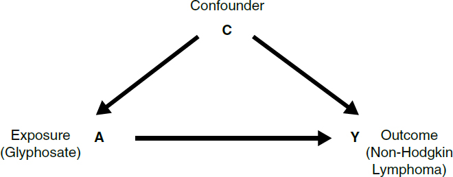
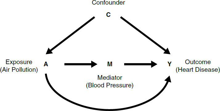
For instance, imagine a hypothetical study of a possible association between exposure to air pollution and risk of heart disease. Based on a review of prior research, the epidemiologist suspects that air pollution may cause heart disease, at least in part, by affecting blood pressure. In this causal model, depicted in a DAG in Figure 7, blood pressure is assumed to mediate, rather than to confound, any causal connection between air pollution and heart disease. The DAG shows that it would be inappropriate to adjust for blood pressure, as this would block the portion of the effect of air pollution that occurs through blood pressure. This example illustrates that adjusting for factors can either remove or introduce bias. Careful examination of the causal relation among factors is necessary to determine the appropriate approach to apply.
Techniques to prevent or limit confounding
Choices in the design of a research project (e.g., methods for selecting the subjects) can prevent or limit confounding. In designing a study, the researcher must determine other risk factors for the disease under study, such as age, sex, or genotype, that may be related to exposure to the agent under study. Investigators can limit the differential distribution of these factors in the study groups by selecting unexposed subjects to “match” exposed subjects in terms of these variables. If the two groups are matched (for example, by age), then any association observed in the study cannot be the result of age, the matched variable.171 Often
171. Selecting a control population based on matched variables necessarily affects the representativeness of the selected controls and may affect how generalizable the study results are to the
investigators frequency-match groups so that the distribution (for example, of age) is similar in the two groups. This reduces the potential for confounding by age but may still require adjustment.
Restricting the persons who are included as subjects in a study is another method to control for confounders. If age or sex is suspected as a confounder, then the subjects enrolled in a study can be limited to those of one sex or those who are within a specified age range. When there is no variance among subjects in a study with regard to a potential confounder, confounding as a result of that variable is eliminated.
In most observational studies, many factors could potentially confound associations. This makes it challenging to apply the matching or restriction methods. Indeed, if age, socioeconomic status, smoking, and race are identified as potential confounders, finding matches or restricting participation to individuals with very precise characteristics may be impractical and make it difficult to generalize findings to individuals with other characteristics than those included in the study. For this reason, most studies use statistical models to control for multiple confounders.
Techniques to control for confounding factors
A good study design will consider potential confounders and obtain data about these variables. There are several analytic approaches to account for the distorting effects of a potential confounder, including stratification or multivariable regression analysis. Stratification permits an investigator to evaluate the effect of a suspected confounder by subdividing the study groups based on a confounding factor. For example, in Table 4, alcohol drinkers have been stratified based on whether they smoke (the suspected confounder).
To take another example that entails a continuous rather than dichotomous potential confounder, let us say we are interested in the relationship between smoking and lung cancer but suspect that air pollution or urbanization may confound the relationship. An observed relationship between smoking and lung cancer could then theoretically be due in part to pollution, if smoking were more common in polluted areas. One could investigate this issue by stratifying the data by degree of urbanization and looking at the relationship between smoking and lung cancer in each urbanization stratum. Figure 8 shows actual
population at large. However, for a study to have merit, it must first be internally valid; that is, it must not be subject to unreasonable sources of bias or confounding. Only after a study has been shown to meet this standard does its universal applicability or generalizability to the population at large become an issue. When a study population is not representative of the general or target population, existing scientific knowledge may permit reasonable inferences about the study’s broader applicability, or additional confirmatory studies of other populations may be necessary.
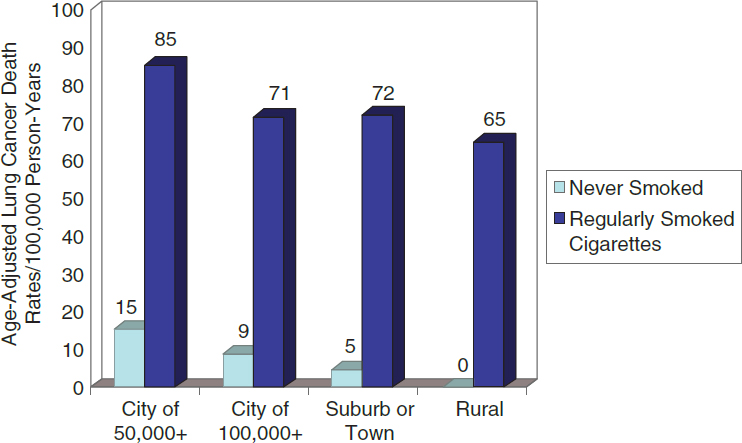 Source: Adapted from E. Cuyler Hammond & Daniel Horn, Smoking and Death Rates: Report on Forty-Four Months of Follow-Up of 187,783 Men: II, Death Rates by Cause, 166 JAMA 1294 (1958).
age-adjusted lung-cancer mortality rates per 100,000 person-years by urban or rural classification and smoking category.172
For each degree of urbanization, lung cancer mortality rates in smokers are shown by the darker bars, and nonsmoker mortality rates are indicated by lighter bars. From these data we see that in every level (or stratum) of urbanization, lung cancer mortality is higher in smokers than in nonsmokers. Therefore, the observed association of smoking and lung cancer cannot be attributed to the level of urbanization. By examining each stratum separately, we, in effect, hold urbanization constant and still find much higher lung cancer mortality in smokers than in nonsmokers.
The standardization method was historically used primarily to control for the effect of age in mortality studies. Two types of standardizations are used—direct and indirect. In direct standardization (e.g., when based on age), overall disease or death rates are calculated for each population as though each had the age distribution of another standard or reference population, using the age-specific disease or death rates for each study population. We can then compare these overall rates, called age-adjusted rates, knowing that any difference
172. This example and Figure 8 (including the source credit in Figure 8) are from Celentano & Szklo, supra note 37, at 294–99.
between these rates cannot be attributed to differences in age, since both age-adjusted rates were generated using the same standard population.
Indirect standardization is used when the age-specific rates for a study population are not known. In that case, the overall disease/death rate for the standard/reference population is recalculated based on the age distribution of the population of interest using the age-specific rates of the standard population. Then, the actual number of disease cases/deaths in the population of interest can be compared with the number in the reference population that would be expected if the reference population had the age distribution of the population of interest.
This ratio is called the standardized mortality ratio (SMR). When the outcome of interest is disease rather than death, it is called the standardized morbidity ratio173 (and the discussion below of standardized mortality rate is equally applicable to a standardized morbidity rate). If the ratio equals 1.0, the observed number of deaths equals the expected number of deaths, and the mortality rate of the population of interest is no different from that of the reference population. If the SMR is greater than 1.0, the population of interest has a higher mortality risk than that of the reference population, and if the SMR is less than 1.0, the population of interest has a lower mortality rate than that of the reference population.
Thus, age adjustment provides a way to compare populations while in effect holding age constant. Adjustment is used not only for comparing mortality rates in different populations but also for comparing rates in different groups of subjects selected for study in epidemiologic investigations. Although this discussion has focused on adjusting for age, it is also possible to adjust for other variables, such as sex, race, genetic variability, occupation, and socioeconomic status.174 However, because this method is based on stratifying study data into groups that will become smaller as the number of variables considered increases, the standardization method can only be used to account for a small number of potential confounders without reducing the numbers in each category to the point at which they are not statistically stable.
As stated above, most studies use statistical models to address multiple confounders at once. Multivariable regression analysis, a technique that relates an outcome to multiple explanatory factors, is most commonly used for this
173. See Burst v. Shell Oil Co., No. CIV.A. 14-109, 2015 WL 3755953, at *6 n.15 (E.D. La. June 16, 2015) (explaining SMR and its relationship with relative risk), aff’d, 650 F. App’x 170 (5th Cir. 2016) (quoting Taylor v. Airco, Inc., 494 F. Supp. 2d 21, 25 n.4 (D. Mass. 2007)). For an example of adjustment used to calculate an SMR for workers exposed to benzene, see Robert A. Rinsky et al., Benzene and Leukemia: An Epidemiologic Risk Assessment, 316 NEJM 1044 (1987), http://doi.org/10.1289/ehp.8982189.
174. For further elaboration on adjustment, see Celentano & Szklo, supra note 37, at 82–85; Cole, supra note 94, at 10,281.
purpose.175 For example, Naranyan and colleagues used logistic regression to estimate whether occupational exposure to pesticides was associated with the risk of Parkinson’s disease in central California while controlling for multiple potential confounders including age, sex, smoking, education, race, and frequency of household pesticide use, as well as ambient residential- and work-address pesticide exposures. In this case-control study, they found that self-reported occupational use of herbicides for a duration exceeding 10 years was associated with a doubling in the risk (i.e., an odds ratio of 2.1 and 95% confidence interval of 1.1 to 3.9) of being diagnosed with Parkinson’s disease.176
However, because there is no free lunch, the use of such methods to address confounding comes at a cost, as they require making a number of assumptions about the characteristics of the data and of the relation among the variables.177 In addition, the larger the number of confounders one wants to control for, the less precise the association between an agent and a disease generally becomes. This is referred to as the bias–variance tradeoff.
The type of multivariable regression model that is used is primarily determined by the form of the outcome data under study. For example, logistic regression (generating odds ratios) is often used for dichotomous outcome data (e.g., presence versus absence of disease); linear regression (generating differences in means) is generally used for continuous outcome data (e.g., blood pressure or IQ); and Cox proportional hazards models (generating hazard ratios) tend to be the method of choice for survival data (e.g., time to death for a given cancer).
Regression analysis was originally developed in the nineteenth century. Statistical methods have evolved, and researchers sometimes use more sophisticated approaches. For example, Bayesian analyses (named after the statistician Thomas Bayes) allow for the integration of prior knowledge in the statistical analysis.178 In a combination between the exposure-matching and the regression
175. For a more complete discussion of multivariable analysis, see Rubinfeld & Card, supra note 31.
176. See Shilpa Narayan et al., Occupational Pesticide Use and Parkinson’s Disease in the Parkinson Environment Gene (PEG) Study, 107 Env’t Int’l 266 (2017), http://doi.org/10.1016/j.envint.2017.04.010.
177. For more details, see Rubinfeld & Card, supra note 31, “What Model Should Be Used to Evaluate the Question at Issue?”
178. Epidemiologic studies assessed by Bayesian statistical analyses have begun to gain a toehold in litigation, although court opinions are still dominated by discussion of traditional significance testing. See In re Abilify (Arpiprazole) Prods. Liab. Litig., No. 3:16MD2734, 2021 WL 4951944, at *5 (N.D. Fla. July 15, 2021) (“Numerous federal courts have found Dr. Madigan’s methodology of detecting safety signals using a combination of frequentist and Bayesian algorithms to be reliable under Rule 702 and Daubert.”); Langrell v. Union Pac. R. Co., No. 8:18CV57, 2020 WL 3037271, at *3 (D. Neb. June 5, 2020) (admitting testimony of specific causation expert who testified “he used a Bayesian approach” to assess causation of a cancer so rare that it was “unlikely or impossible for epidemiological studies to be performed”); In re Testosterone Replacement Therapy Prods. Liab. Litig., No. 14 C 1748, 2018 WL 4030585, at *8 (N.D. Ill. Aug. 23, 2018) (denying motion to exclude testimony of expert “whose Bayesian critiques of epidemiological studies” were similar to those of another expert whose testimony “the Court has previously found admissible”). For a description of
approaches, propensity score matching allows researchers to match study subjects based on their probability of exposure given the value of potential confounders.179 The potential outcome (or counterfactual) approach aims to simulate randomized-controlled trials by estimating outcomes under different exposure scenarios in which measured confounders are not related to the exposure and/or the outcome. Methods applying this approach include inverse-probability weighting and the parametric g-formula.
The methods described above, through different means and under different assumptions, allow for adjustment of the effect of confounders on an association between an agent and a disease. They aim to estimate the association after having removed confounding by the measured variables. The details of these methods are too technical for discussion here. The crucial points to recognize are that using statistical models to address possible confounding is an accepted part of epidemiologic practice and that choosing the correct statistical model for a study is important to the validity of the study’s results. If an association between an agent and a disease remains after accounting for selection, information, and confounding bias, a researcher must then assess whether an inference of causation is justified. This entails consideration of the Hill factors explained in the section below titled “General Causation.”
Conceptual Error
In addition to the possibility of bias, a study may also be limited by flawed definitions or premises in its design. Consider, for example, a researcher who wishes to investigate whether a certain drug is teratogenic (causes birth defects). If the researcher defines the disease of interest as all birth defects, rather than a specific type of birth defect, there should be a scientific basis to hypothesize that the effects of the drug could be so broad. If the effect is in fact more limited, the result of this conceptualization error could be to dilute or mask any real effect that the agent might have on a specific type of birth defect.180
Bayesian statistical methods, see Kaye & Stern, supra note 16, “Bayesian Statistical Methods and Posterior Probabilities” and “Appendix: Conditional Probability and Bayes’ Rule.”
179. “Propensity scoring is a system where researchers attempt to control for confounding by creating a comorbidity ‘score’ for a study participant; the more confounding comorbidities a participant has, the higher [the participant’s] score and, through the score, the researchers estimate the propensity of the subject to contribute to confounding.” In re Zantac (Ranitidine) Prods. Liab. Litig., 644 F. Supp. 3d 1075, 1260 (S.D. Fla. 2022). In Zantac, the court excluded proffered expert testimony in part because the court found that the experts testified inconsistently about the merits of propensity scoring. Id. at 1261.
180. In Brock, 874 F.2d at 312, the court discussed a reanalysis of a study in which the effect was narrowed from all congenital malformations to limb-reduction defects. The magnitude of the association changed by 50% when the effect was defined in this narrower fashion. See Timothy J. Lash et al., Measurement and Measurement Error, in Lash et al., supra note 50, at 287, 297
Similarly, if the researcher studies the connection between the drug and limb-reduction birth defects in particular, the researcher should consider that an exogenous agent can only cause such a defect during the period of limb organogenesis (weeks 5–9 of the pregnancy). If the researcher defines exposure as the mother taking the drug anytime during her pregnancy, conceptual bias is introduced. Classifying as exposed those pregnant women who took the drug outside the window when exposure could have caused the outcome of interest would tend to understate any association that might exist.
Biases That Affect a Body of Epidemiologic Evidence
Some biases go beyond errors in individual studies and affect the overall body of available evidence in a way that skews what appears to be the universe of evidence. Publication bias is the tendency for scientific journals to prefer to publish studies that find an association.181 If negative studies are never published, the published literature as a whole will be biased. These types of biases may present problems for researchers who attempt to synthesize or combine the results of multiple studies to assess the existence and magnitude of an association.182
Financial conflicts of interest by researchers and the source of funding of studies have also been shown to have an effect on the outcomes of such studies.183 As the former editor-in-chief of the British Medical Journal noted:
(“Unwarranted assurances of a lack of any effect can easily emerge from studies in which a wide range of etiologically unrelated outcomes are grouped.”). For a more general discussion of conceptualization and other types of errors and their relation to legal decision-making, see Vern R. Walker, Theories of Uncertainty: Explaining the Possible Sources of Error in Inferences, 22 Cardozo L. Rev. 1523, 1544–47, 1553–55 (2001).
181. Celentano & Szklo, supra note 37, at 234. Investigators may contribute to this effect by neglecting to submit negative studies for publication. Publication bias “can pose a serious problem when the results from all published clinical trials are reviewed.” Id. Publication bias can also affect systematic reviews or meta-analyses of observational studies on a given agent–disease relationship. For clinical trials, medical journals have attempted to minimize publication bias by requiring that before any study is considered for publication, it must have been registered in a public trial registry before any data is gathered. See Catherine D. DeAngelis et al., Clinical Trial Registration: A Statement from the International Committee of Medical Journal Editors, 292 JAMA 1363 (2004), https://doi.org/10.1056/NEJMe048225. The National Institutes of Health (NIH) requires that all NIH-funded clinical trials must be registered and the results reported. See Nat’l Insts. of Health, NIH Policy on the Dissemination of NIH-Funded Clinical Trial Information, NOT-OD-16-149, Sept. 16, 2016, https://grants.nih.gov/grants/guide/notice-files/NOT-OD-16-149.html.
182. See section titled “Methods for Synthesizing or Combining the Results of Multiple Studies” below.
183. See Jerome P. Kassirer, On the Take: How Medicine’s Complicity with Big Business Can Endanger Your Health 79–84 (2005); Deepa V. Cherla et al., The Effect of Financial Conflict of Interest, Disclosure Status, and Relevance on Medical Research from the United States, 34 J. Gen. Internal Med.
The major determinant of whether reviews of passive smoking concluded it was harmful was whether the authors had financial ties with tobacco manufacturers. In the disputed topic of whether third-generation contraceptive pills cause an increase in thromboembolic disease, studies funded by the pharmaceutical industry find that they don’t and studies funded by public money find that they do.184
Effect Modification
Populations and individuals with different characteristics may be more or less susceptible to the adverse health effects of an agent. Such characteristics are called effect modifiers.
For example, sex and gender are suspected to modify the effect of a number of associations. Stronger associations between exposure to air pollution and respiratory outcomes have been reported among women relative to men.185 Biologic sex may also modify associations between exposure to agents, such as pesticides and hormones, and some health outcomes.186 Age may also modify associations. For example, associations between an agent and age may occur if
429 (2019), https://doi.org/10.1007/s11606-018-4784-0; Adam G. Dunn et al., Conflict of Interest Disclosure in Biomedical Research: A Review of Current Practices, Biases, and the Role of Public Registries in Improving Transparency, 1 Rsch. Integrity & Peer Rev. 1 (2016), https://doi.org/10.1186/s41073-016-0006-7.
Epidemiologists, like other scientists, also may engage in scientific misconduct, even fraud. See generally James R. Wible, The Economics of Scientific Misconduct 24–38 (2023) (describing two “waves” of scientific misconduct in the late 20th and early 21st centuries and reviewing studies attempting to estimate how often misconduct occurs); Steven L. George, Research Misconduct and Data Fraud in Clinical Trials: Prevalence and Causal Factors, 21 Int’l J. Clinical Oncology 15, 16 (2016), https://doi.org/10.1007/s10147-015-0887-3 (listing several instances of falsified or fabricated data in clinical trials); Steven S. Coughlin et al., Ethics and Scientific Integrity in Public Health, Epidemiological and Clinical Research, 34 Pub. Health Rev. 1, 6 (2012), https://doi.org/10.1007/BF03391657 (providing example of published falsified epidemiologic data); Ferric Fang et al., Misconduct Accounts for the Majority of Retracted Scientific Publications, 42 PNAS 17028, 17029 (2012) (“nearly half of retractions are for fraud or suspected fraud”); Douglas L. Weed, Preventing Scientific Misconduct, 88 Am. J. Pub. Health 125, 126 (1998), https://doi.org/10.2105/ajph.88.1.125 (noting that although the frequency of scientific misconduct is difficult to quantify, “big effects may arise from small numbers”). Courts should be aware of this possibility, although in an adversarial system, the opposing party has the primary role in identifying such misbehavior when it could have an impact on the case at hand. In-depth discussion of scientific misconduct is beyond the scope of this guide.
184. Richard Smith, Making Progress with Competing Interests, 325 BMJ 1375, 1376 (2002), https://doi.org/10.1136/bmj.325.7377.1375.
185. See Jane Clougherty, A Growing Role for Gender Analysis in Air Pollution Epidemiology, 118 Env’t Health Persps. 167 (2010), https://doi.org/10.1289/ehp.0900994.
186. See Jonathan Chevrier et al., Sex and Poverty Modify Associations Between Maternal Peripartum Concentrations of DDT/E and Pyrethroid Metabolites and Thyroid Hormone Levels in Neonates Participating in the VHEMBE Study, 131 Env’t Int’l 131 (2019), https://doi.org/10.1016/j.envint.2019.104958.
older individuals are more likely than younger individuals to develop a particular disease (such as cancer) after exposure to the agent.
Exogenous agents may serve as effect modifiers as well. One example involves warfarin, a drug used to prevent clotting in individuals at risk of strokes and other blood-mediated adverse outcomes. A case study reported on a woman whose measure of the effect of warfarin on her blood clotting, known as the international normalized ratio (INR), was stable but whose INR became doubled when she drank cranberry juice. Her INR returned to normal when she ceased drinking cranberry juice.187 Cranberry juice thus appears to be an effect modifier for the anti-coagulation effects of warfarin.
Susceptibility to a given exposure may also be modified by genetic factors, a concept known as gene–environment interaction. For example, while smoking is a known risk factor for bladder cancer, a meta-analysis188 found that the relative risk was 40% greater among individuals who eliminate some chemicals more slowly owing to a particular variant of the gene NAT2, relative to those with other variants of the gene who eliminate chemicals faster.189
Genetic variations190 that affect how toxicants are metabolized, and therefore affect the effects of exposures on disease risks, may be common.191 To the
187. See Gale L. Hamann et al., Warfarin-cranberry juice interaction, 45(3) Ann. Pharmacotherapy e17 (2011), https://doi:10.1345/aph.1P451.
188. See section titled “Methods for Synthesizing or Combining the Results of Multiple Studies” below.
189. See Montserrat García-Closas et al., NAT2 Slow Acetylation, GSTM1 Null Genotype, and Risk of Bladder Cancer: Results from the Spanish Bladder Cancer Study and Meta-Analyses, 366 Lancet 649 (2005), https://doi.org/10.1016/S0140-6736(05)67137-1.
190. A gene is a segment of DNA that, through its sequence of components called bases, codes for the production of a protein or part of a protein. Genetic variations are alterations in the sequence of bases that constitute a person’s DNA. These variations may be present in the sperm and egg cells that join to form an embryo (germline mutations), in which case they affect all of a person’s cells, or they may arise at some point during life (somatic mutations), in which case they affect only cells descended from cells in which the change occurred. DNA may vary in many different ways. A frequently studied type of genetic variation is a polymorphism—a segment of DNA that occurs in multiple forms (alleles) in the population as a result of inherited mutations in some portion of the base sequence. Polymorphisms may affect the structure or function of the protein encoded by a gene and may therefore affect health. In addition to changes in the genetic structure itself, epigenetic changes—alterations in the molecules that control the extent of gene expression (protein production)—may affect how the body interacts with potential toxicants. See, e.g., McMillan v. Togus Regional Off., Dep’t of Veterans Affs., 294 F. Supp. 2d 305, 312 (E.D.N.Y. 2003) (“It is generally accepted that genetic susceptibility plays a key role in determining the adverse effects of environmental chemicals. . . . [I]f polymorphisms of the gene encoding the AhR [protein] exist in humans as they do in laboratory animals, some people would be at greater risk or at lesser risk for the toxic and carcinogenic effects of TCDD [dioxin].”)
191. See Ebony B. Bookman et al., Gene–Environment Interplay in Common Complex Diseases: Forging an Integrative Model: Recommendations from an NIH Workshop, 35 Genetic Epidemiology 217, 218–19 (2011), https://doi.org/10.1002/gepi.20571 (stating that susceptibility to most human diseases “is complex and multifactorial” and describing the difficulty of assessing risk contribution in
extent that genetic variability is reflected in risk heterogeneity, an epidemiologic study that does not consider its subjects’ genotypes in addition to their exposure status may produce results that are not entirely valid with respect to some portion of the study participants, even if the study validly reports the relative risk of exposure for the study sample as a whole.192 The study might understate the relative risk for people whose genetics make them more vulnerable to the effects of the exposure (perhaps even to the point of finding no association at all in the sample as a whole) and overstate the relative risk for people whose genetics protect them from the effects of the exposure. This does not mean that epidemiologic studies must consider genetic variability in order to provide useful causal evidence. Currently, most epidemiologic studies do not gather detailed genetic information on the study participants193 for various reasons, including incomplete current scientific understanding of genetic differences in susceptibility to exposure.194
gene-environment interactions); Frederica P. Perera, Molecular Epidemiology: On the Path to Prevention?, 92 J. Nat’l Cancer Inst. 602, 608 (2000), https://doi.org/10.1093/jnci/92.8.602 (“new molecular epidemiologic and other data invalidate the assumption of population homogeneity”); see also, e.g., Brenda Eskenazi et al., Organophosphate Pesticide Exposure, PON1, and Neurodevelopment in School-Age Children from the CHAMACOS Study, 134 Env’t Rsch. 149, 156 (2014), https://doi.org/10.1016/j.envres.2014.07.001 (“Future policies regarding protection from [organophosphate] pesticide exposure should consider that some children may be more vulnerable to early life exposures by virtue of their or their mother’s genetic predispositions. . . .”).
192. The relative risk for the population as a whole will depend on the relative risk of exposure for each relevant genotype and the frequency of each relevant genotype in the population. Either of these values might be inaccurately measured in a study, either because of random error or because of some type of bias (e.g., a sample of people of one ancestry might not accurately reflect the genotype frequencies in a more diverse population).
193. See Witte & Thomas, supra note 50, at 964 (“The incorporation of environmental factors into studies of genetics has been slower moving. While some complex diseases have long been recognized as having both environmental and familial components, our understanding of their interaction is only in its infancy. . . . much remains to be understood.”).
194. Even if, for instance, a study shows that the relative risk associated with an exposure varies with different variants of a particular gene, variants affecting the relative risk could also exist in other genes. The study might or might not assess what those other genes are and how differences in the various involved genes interact with each other. The biological effects of exposure to benzene, for example, appear to be influenced by variations in at least five genes. See Diana Dougherty et al., NQO1, MPO, CYP2E1, GSTT1 and GSTM1 Polymorphisms and Biological Effects of Benzene Exposure—A Literature Review, 182 Toxicology Letters 7, 15 (2008) (“this review shows that multiple genetic polymorphisms on the benzene metabolism pathway should be taken into account when studying the biological effects of benzene exposure”). Studies have also identified several genes with variants that are associated with different relative risks for tobacco smokers of both lung cancer, see Boffetta, supra note 57, at 124, and chronic obstructive pulmonary disease, see Chimedikhamsuren Ganbold et al., The Cumulative Effect of Gene-Gene Interactions Between GSTM1, CHRNA3, CHRNA5 and SOD3 Gene Polymorphisms Combined with Smoking on COPD Risk, 16 Int’l J. Chronic Obstructive Pulmonary Disease 2857, 2866 (2021), https://doi.org/10.2147/COPD
Although some courts have considered general claims of differential susceptibility to toxic exposures,195 few have been confronted with epidemiologic studies that quantitatively assess the degree to which an association between disease risk and exposure status appears to have been modified by genetic variability.196 It is reasonable to believe that courts will see more such studies197 offered as evidence on the issue of general causation.198 If that occurs, knowledge of the plaintiff’s genotype could be relevant,199 although not necessarily essential, evidence on the issue of specific causation.200
.S320841/ (“few studies consider gene-gene or gene-environment interaction with the genetic factors in COPD susceptibility”).
195. See, e.g., In re Asbestos Prods. Liab. Litig., No. 10-CV-61118, 2011 WL 605801 (E.D. Pa. Feb. 16, 2011) (denying motion to exclude testimony of expert witness who opined “that susceptibility to asbestos-related disease varies within the population and the dose of asbestos necessary to cause the disease is different for each individual, and largely dependent upon genetic predisposition”); Young v. Burton, 567 F. Supp. 2d 121, 137 (D.D.C. 2008) (rejecting plaintiff’s expert’s claim that variations in HLA-DR gene affected susceptibility to illness resulting from exposure to mold); Blackwell v. Wyeth, 971 A.2d 235, 252–53 (Md. 2009) (affirming exclusion of expert testimony that mercury in vaccine caused autism in genetically susceptible plaintiff where trial judge found no evidence that the genetic variants about which the expert testified were associated with autism or affected mercury excretion).
196. Genetic variation in susceptibility to the toxic effects of beryllium was central to Sheridan v. NGK Metals Corp., 609 F.3d 239, 244 (3d Cir. 2010), “because only persons who have a particular genetic ‘marker’—the Human Leukocyte Antigen (HLA)-DPB1 allele—can potentially recognize beryllium in the lungs as an antigen.” The court observed that “[m]ultiple studies have attempted to determine the percentage of the population that is genetically predisposed, or ‘susceptible,’ to [chronic beryllium disease]. The results so far are inconclusive and disputed.” Id. at 245; see also Paz v. Brush Engineered Metals, Inc., 555 F.3d 383, 396 n.22 (5th Cir. 2009) (quoting an expert witness’s article stating that from 1% to 16% of individuals exposed to beryllium develop disease, depending on genetic susceptibility and nature of exposure).
197. See generally, e.g., Cosetta Minelli et al., Interactive Effects of Antioxidant Genes and Air Pollution on Respiratory Function and Airway Disease: A HuGE Review, 173 Am. J. Epidemiology 603, 618 (2011), https://doi.org/10.1093/aje/kwq403 (“The study of genetic susceptibility can greatly improve our understanding of air pollution pathophysiologic mechanisms of action and allow identification of those pollution components with the highest potential for harm.”).
198. See section titled “General Causation” below for a discussion of general causation.
199. See Spahn v. Sec’y of Health & Hum. Servs., 133 Fed. Cl. 588, 593, 600 (Fed. Cl. 2017) (sustaining special master’s rejection of claim for compensation for vaccine injury where claimant’s expert opined that CPOX4 mutation rendered claimant ultra-susceptible to neurotoxic effects of mercury in the vaccine but claimant did not undergo genetic testing to determine whether he had the mutation).
200. Consider, hypothetically, a gene that occurs in two forms (alleles), A and a; people with at least one A allele (genotype AA or Aa) who are exposed to toxicant T have a relative risk of 10 for a particular disease, but exposed people without an A allele (genotype aa) are protected from the toxicity and have a relative risk of 1 (no association). An exposed AA or Aa plaintiff would have a different case from an exposed aa plaintiff. But suppose that a alleles are rare, so that aa genotypes account for only 1% of the population. It might be reasonable to permit the factfinder to draw the inference that a sick, exposed plaintiff was not aa, even if the plaintiff’s actual
To illustrate effect modification, below are hypothetical data from a case-control study for the relationship of a dichotomous exposure, such as smoking (ever vs. never), and a dichotomous outcome, such as the existence of a disease. The data reveal effect modification by sex.
TOTAL
| Diseased | Not diseased | Total | |
|---|---|---|---|
| Exposed | 300 | 250 | 550 |
| Not Exposed | 200 | 250 | 450 |
The odds ratio for the association between exposure and disease for the total sample (males and females together) is 1.50; statistical analysis reveals a 95% confidence interval (CI) bounded by 1.20 and 1.90 and a p-value equaling 0.002 (often abbreviated as “95% CI = 1.20, 1.90; p = 0.002”). The low p-value means that this association is statistically significant for the entire study sample. However, we may have reason to believe that the exposure may differentially affect males and females. To examine this possibility, we stratify the data by sex.
MALES
| Diseased | Not diseased | Total | |
|---|---|---|---|
| Exposed | 80 | 50 | 130 |
| Not Exposed | 45 | 75 | 120 |
The odds ratio for the association between exposure and disease in the males is 2.70 (95% CI = 1.60, 4.60, p < 0.001). The low p-value means that this association is statistically significant, but the relatively wide confidence interval reflects the moderate size of the subsample of males (n = 250).
FEMALES
| Diseased | Not diseased | Total | |
|---|---|---|---|
| Exposed | 220 | 200 | 420 |
| Not Exposed | 155 | 175 | 330 |
genotype for some reason cannot be ascertained. Alternatively, limitations of the genetic epidemiology studies themselves, see supra note 53 and accompanying text, might affect the probative value of evidence of the plaintiff’s genotype. Specific causation is discussed in the section titled “Specific Causation” below.
The odds ratio for the association between exposure and disease in the females is 1.20 (95% CI = 0.90, 1.70, p = 0.14). The higher p-value means that this association is not statistically significant and the narrower confidence interval relative to males reflects the larger size of the subsample of females (n = 750).
We can test for whether the association between exposure and outcome is statistically different among males (OR = 2.70) relative to females (OR = 1.20). The p-value for the interaction is small (0.01), i.e., the interaction is statistically significant, suggesting that the finding that sex modifies the association between the exposure and the disease is not likely the result of random error.201
General Causation
Once epidemiologists conclude that an association exists, the next question is whether an inference of causation is appropriate.202 To make a judgment about causation, a knowledgeable expert considers the available studies and evaluates the body of evidence using the criteria described below.203
201. One court quoted an expert witness who explained the importance of effect modification thusly: “‘If, for example, the association between an exposure and an outcome is different for men than for women, sex modifies the relationship between the exposure and the outcome.’ . . . When effect modification is present, ‘[c]ombining the two groups to create a summary measure of association is meaningless: it is not true for men and it is not true for women.’” Ohio Valley Env’t Coal. v. Fola Coal Co., 120 F. Supp. 3d 509, 520–21 (S.D. W. Va. 2015) (quoting epidemiologist David Garabrandt; citations omitted).
Effect modification can coexist with confounding (see the section titled “Confounding Bias” above). Using slightly different terminology, one epidemiology textbook explained:
Effect-measure modification differs from confounding in several important ways. The most salient difference is that, whereas confounding is a bias that the investigator hopes to prevent or remove from the effect estimate, effect-measure modification is a property of the effect under study. Thus, effect-measure modification is a finding to be reported rather than a bias to be avoided or removed. Moreover, in epidemiologic analysis, one tries to eliminate confounding, but one may be interested in describing effect-measure modification. Sebastien Haneuse & Kenneth J. Rothman, Stratification and Standardization, in Lash et al., supra note 50, at 609, 610.
202. For an excellent example of the authors of a study analyzing whether an inference of causation is appropriate in a case-control study examining whether bromocriptine (Parlodel) (a lactation suppressant) causes seizures in postpartum women, see Kenneth J. Rothman et al., Bromocriptine and Puerperal Seizures, 1 Epidemiology 232, 236–38 (1990), https://doi.org/10.1097/00001648-199005000-00009.
203. In a lawsuit, this would be done by an expert witness. In science, the effort is usually conducted by a panel of experts. See Douglas L. Weed, Epidemiologic Evidence and Causal Inference, 14 Hematology/Oncology Clinics N. Am. 797 (2000) (discussing judgment involved in selecting criteria and assigning rules of evidence to them in the process of judging whether an association is causal); Restatement (Third) of Torts: Liability for Physical and Emotional Harm § 28 cmt. c (2010) (“[A]n evaluation of data and scientific evidence to determine whether an inference of causation is appropriate requires judgment and interpretation.”).
When epidemiologists evaluate whether a cause–effect relationship exists between an agent and a health outcome, they are using the term causation in a way similar, but not identical, to the way that the familiar but-for, or sine qua non, test is used in law for cause in fact. “Conduct is a factual cause of [harm] when the harm would not have occurred absent the conduct.”204 This is equivalent to describing the act or occurrence as a necessary link in a chain of events that results in the particular outcome.205 Epidemiologists use causation to mean that an increase in the incidence of disease or an adverse health outcome among the group of exposed subjects would not have occurred had they not been exposed to the agent.206 Thus, exposure is a necessary condition for the increase in the incidence of disease among those exposed.207 The relationship between the epidemiologic concept of cause and the legal question of whether exposure to an agent caused an individual’s disease is addressed in the section below titled “Specific Causation.”
Data from epidemiologic studies, as well as from toxicology and in vitro studies, are also considered in an approach termed weight of evidence.208 In the landmark 1964 Surgeon General’s report on smoking and health, smoking was determined to be a causal agent in lung cancer based on the consistency, strength,
More generally, causation always requires an inference from circumstantial evidence because causation cannot be perceived directly with any of the five senses. Epidemiologic evidence is one form of circumstantial evidence that informs the inferential process when the causal question involves agents and disease.
204. Restatement (Third) of Torts: Liability for Physical and Emotional Harm § 26 (2010); see also Dan B. Dobbs et al., Dobbs’ Law of Torts § 189 (updated 2024). When multiple causes are each operating and each is independently capable of causing an event, the but-for, or necessary-condition, concept for causation is problematic. This is the familiar two-fires scenario, in which two independent fires simultaneously burn down a house and is sometimes referred to as overdetermined outcomes. Neither fire is a but-for, or necessary condition, for the destruction of the house, because either fire would have destroyed the house. See Restatement (Third) of Torts: Liability for Physical and Emotional Harm § 28 (2010). This two-fires situation is analogous to an individual being exposed to two agents, each of which is capable of causing the disease contracted by the individual. See Basko v. Sterling Drug, Inc., 416 F.2d 417 (2d Cir. 1969).
205. See supra note 10; see also Restatement (Third) of Torts: Liability for Physical and Emotional Harm § 26 cmt. c (2010) (employing a “causal set” model to explain multiple elements, each of which is required for an outcome).
206. Bruce G. Charlton, Attribution of Causation in Epidemiology: Chain or Mosaic?, 49 J. Clinical Epidemiology 105, 105 (1999), https://doi.org/10.1016/0895-4356(95)00030-5 (“The imputed causal association is at the group level, and does not indicate the cause of disease in individual subjects.”).
207. See Lash et al., supra note 50, at 8 (“We can define a cause of a specific disease event as an antecedent event, condition, or characteristic that was necessary for the occurrence of the disease at the moment it occurred, given that other conditions are fixed.”); Allen v. United States, 588 F. Supp. 247, 405 (D. Utah 1984) (quoting a physician on the meaning of the statement that radiation causes cancer), rev’d on other grounds, 816 F.2d 1417 (10th Cir. 1987).
208. See supra note 71 and accompanying text.
specificity, temporal relationship, and coherence of the association.209 A year later, Sir Austin Bradford Hill published a list of elements to consider for inferring causation from an association that partially overlapped with those applied in the Surgeon General’s report.210 The items Hill identified are sometimes erroneously presented as mandatory “criteria” rather than as factors or considerations, but Hill himself acknowledged that they could only serve to assist in the inferential process: “None of my nine viewpoints can bring indisputable evidence for or against the cause-and-effect hypothesis and none can be required as a sine qua non.”211 Yet it is imperative to note that epidemiologists employ these guidelines only after a study finds an association, to determine whether that association reflects a true causal relationship.212 These guidelines consist of several key inquiries that assist researchers in making a judgment about causation.213 Generally, researchers are conservative when it comes to assessing causal relationships, often calling for stronger evidence and more research before a conclusion of causation is drawn.214
209. U.S. Dep’t Health, Educ. & Welfare, Pub. Health Serv., Smoking and Health: Report of the Advisory Committee to the Surgeon General of the Public Health Service 26–32 (1964) (describing the types of evidence considered in reaching the report’s conclusion), https://perma.cc/9TH2-JP7B.
210. See Austin Bradford Hill, The Environment and Disease: Association or Causation?, 58 Proc. Royal Soc’y Med. 295 (1965). For discussion of these considerations and their respective strengths in informing a causal inference, see Celentano & Szklo, supra note 37, at 236–39; David E. Lilienfeld & Paul D. Stolley, Foundations of Epidemiology 276–80 (3d ed. 2019); Weed, supra note 203.
211. See Hill, supra note 210, at 36.
212. In a number of cases, experts attempted to use these guidelines to support the existence of causation in the absence of any epidemiologic studies finding an association. Compare Rains v. PPG Indus., 361 F. Supp. 2d 829, 836–37 (S.D. Ill. 2004) (explaining Hill factors and proceeding to apply them even though there was no epidemiologic study that found an association) and Wendell v. GlaxoSmithKline LLC, 858 F.3d 1227, 1235–36 (9th Cir. 2017) (reversing exclusion of testimony of plaintiff’s expert who “used the Bradford Hill methodology” but “did not rely on animal or epidemiological studies”) with Hoefling v. U.S. Smokeless Tobacco Co., 576 F. Supp. 3d 262, 273 (E.D. Pa. 2021) (finding an expert’s general causation opinion based on the Hill factor of “biological plausibility” unreliable because there was no epidemiologic evidence supporting an association), In re Roundup Prods. Liab. Litig., 390 F.3d 1102, 1131 (N.D. Cal. 2018) (“identifying an association . . . is a necessary predicate to reliable application of the Bradford Hill criteria”), and Jones v. Novartis Pharms. Corp., 235 F. Supp. 3d 1244, 1268 (N.D. Ala. 2017) (inability to point to a study showing an association between exposure and disease was “fatal flaw” of expert’s reliance on Hill factors (citing the third edition of this reference guide)).
213. See Mervyn Susser, Causal Thinking in the Health Sciences: Concepts and Strategies in Epidemiology (1973); Gannon v. United States, 571 F. Supp. 2d 615, 624 (E.D. Pa. 2007) (quoting expert who testified that the Hill factors are “‘well-recognized’ and widely used in the science community to assess general causation”); Chapin v. A & L Parts, Inc., 732 N.W.2d 578, 584 (Mich. Ct. App. 2007) (expert testified that Hill factors are the most well-utilized method for determining if an association is causal).
214. Berry v. CSX Transp., Inc., 709 So. 2d 552, 568 n.12 (Fla. Dist. Ct. App. 1998) (“Almost all genres of research articles in the medical and behavioral sciences conclude their discussion with qualifying statements such as ‘there is still much to be learned.’ This is not, as might be assumed, an expression of ignorance, but rather an expression that all scientific fields are open-ended and can
Some regulatory agencies have modified the Hill factors in a number of ways and used them as a guide. The United States Environmental Protection Agency (EPA) has employed a system called the Causal Analysis/Diagnosis Decision Information System, or CADDIS, a weight-of-evidence approach to identify causal agents.215 The International Agency for Research on Cancer (IARC) also relies on a weight-of-evidence approach that considers epidemiologic studies, animal experiments, and mechanistic information.216 The IARC convenes groups of experts in various fields who are asked to reach consensus and to collectively consider the strength of the association, consistency across studies and diverse populations, dose–response relationships, biological plausibility, and temporal relationships observed in epidemiologic studies, as well as the results of animal and mechanistic studies.217
The following is a modified list of the Hill considerations218 that inform epidemiologists in making judgments about causation (there is no threshold number that must exist219):
- Temporal relationship
- Strength of the association
progress from their present state. . . .”); Hall v. Baxter Healthcare Corp., 947 F. Supp. 1387, 1446–51 (D. Or. 1996) (report of Merwyn R. Greenlick, court-appointed epidemiologist). In Cadarian v. Merrell Dow Pharms., Inc., 745 F. Supp. 409 (E.D. Mich. 1989), the court refused to permit an expert to rely on a study that the authors had concluded should not be used to support an inference of causation in the absence of independent confirmatory studies. The court did not address the question whether the degree of certainty used by epidemiologists before making a conclusion of cause was consistent with the legal standard. See DeLuca, 911 F.2d at 957 (standard of proof for scientific community is not necessarily appropriate standard for expert opinion in civil litigation); Wells v. Ortho Pharm. Corp., 788 F.2d 741, 745 (11th Cir. 1986).
215. U.S. Env’t Prot. Agency, Causal Analysis/Diagnostic Decision Information System (CADDIS), https://perma.cc/2L4R-58T8 (last visited Aug. 5, 2024); see U.S. Env’t Prot. Agency, CADDIS Volume 1: Stressor Identification—About Causal Assessment, “An Approach to Causal Inference,” https://perma.cc/T52H-X84S (“We accept multiple causation concepts and all relevant evidence and methods for turning data into evidence.”).
216. For a discussion of mechanistic data, see Eaton et al., supra note 60, “Toxicological Processes and Target Organ Toxicity.”
217. See generally, e.g., Int’l Agency for Rsch. on Cancer, 96 IARC Monographs on the Evaluation of Carcinogenic Risks to Humans: Alcohol Consumption and Ethyl Carbamate 7–33 (2010) (describing IARC approach).
218. This list was developed by Leon Gordis, the epidemiologist coauthor of the first three editions of this reference guide. See Celentano & Szklo, supra note 37, at 276–79. The original Hill considerations were: 1) consistency; 2) strength; 3) specificity; 4) dose–response; 5) temporal relationship; 6) biological plausibility; 7) coherence; and 8) experiment. See Hill, supra note 210. These considerations are largely congruent with the factors listed in the text, although with some wording differences and the addition of the “consideration of alternative explanations” item in the text.
219. See Cook v. Rockwell Int’l Corp., 580 F. Supp. 2d 1071, 1098 (D. Colo. 2006) (“Defendants cite no authority, scientific or legal, that compliance with all, or even one, of these factors is required . . . The scientific consensus is, in fact, to the contrary. It identifies Defendants’ list of factors as some of the nine factors or lenses that guide epidemiologists in making judgments about causation . . . These factors are not tests for determining the reliability of any study or the causal inferences drawn from it.”).
- Dose–response relationship
- Replication of the findings
- Biological plausibility
- Consideration of alternative explanations
- Cessation of exposure
- Specificity of the association
- Consistency with other relevant knowledge
There is no formula or algorithm that can be used to assess whether a causal inference is appropriate based on these guidelines.220 One or more factors may be absent even when a true causal relationship exists.221 Similarly, the existence of some factors does not ensure that a causal relationship exists. Drawing causal inferences after finding an association and considering these factors requires judgment and searching analysis, based on biology, of why a factor or factors may be absent despite a causal relationship, and vice versa. Although the drawing of causal inferences is informed by scientific expertise, it is not a determination that is made by using an objective or algorithmic methodology.222
Temporal Relationship
A temporal, or chronological, relationship must exist for causation to exist. If an exposure causes disease, the exposure must occur before the disease develops.223 If the exposure occurs after the disease develops, it cannot have caused the disease. Although temporal relationship is often listed as one of many factors in assessing whether an inference of causation is justified, this aspect of a temporal relationship is a necessary factor: Without exposure before the disease, causation cannot exist.224
220. See Douglas L. Weed, Epidemiologic Evidence and Causal Inference, 14 Hematology/Oncology Clinics N. Am. 797 (2000), https://doi.org/10.1016/s0889-8588(05)70312-9.
221. See Cook v. Rockwell Int’l Corp., 580 F. Supp. 2d 1071, 1098 (D. Colo. 2006) (rejecting argument that plaintiff failed to provide sufficient evidence of causation based on failing to meet four of the Hill factors).
222. See David A. Savitz & Gregory Wellenius, Interpreting Epidemiologic Evidence: Study Design and Analysis 199–210 (2d ed. 2016).
223. See McClain v. Metabolife Int’l, Inc., 401 F.3d 1233, 1243 (11th Cir. 2005) (“‘[T]he chronological relationship between exposure and effect must be biologically plausible . . . [thus], if a disease or illness in an individual preceded the established period of exposure, then it cannot be concluded that the chemical caused the disease, although it may be possible to establish that the chemical aggravated a pre-existing condition or disease.’”) (quoting David L. Eaton, Scientific Judgment and Toxic Torts: A Primer in Toxicology for Judges and Lawyers, 12 J. L. & Pol’y 5 (2003)).
224. However, exposure during the disease initiation process may cause the disease to be more severe than it otherwise would have been without the additional dose.
With specific causation, a subject dealt with in detail in the section below titled “Specific Causation,” there may be circumstances in which a temporal relationship supports the existence of a causal relationship.
If the latency period between exposure and outcome is known,225 then exposure consistent with that information may lend credence to a causal relationship. This is particularly true when the latency period is short and competing causes are known and can be ruled out. Thus, if an individual suffers an acute respiratory response shortly after exposure to a suspected agent, and other causes of that respiratory problem are known and can be ruled out, the temporal relationship strongly supports the conclusion that a causal relationship exists.226 By contrast, exposure outside a known latency period, such as an exposure very quickly followed by development of cancer, constitutes evidence against the existence of causation.227 When latency periods are lengthy, variable, or not known, and a substantial proportion of the disease is due to unknown causes, temporal relationship provides little beyond satisfying the requirement that cause precede effect.228
225. When the latency period is known—or is known to be limited to a specific time period—as is the case with the adverse effects of some vaccines—the time frame from exposure to manifestation of disease can be critical to determining causation. Thus, epidemiologic evidence identified the swine flu vaccine as a cause of Guillain-Barre syndrome (GBS) but the peak latency period was two to three weeks after vaccination and the excess risk disappeared after 10 weeks. That evidence was critical in denying recovery to a swine flu vaccinee who developed GBS 17 weeks after vaccination. See Robinson v. United States, 533 F. Supp. 320, 328 (E.D. Mich. 1982).
226. For courts that have relied on temporal relationships of the sort described, see Bonner v. ISP Technologies, Inc., 259 F.3d 924, 930–31 (8th Cir. 2001) (giving more credence to the expert’s opinion on causation for acute response based on temporal relationship than for chronic disease that plaintiff also developed); Heller v. Shaw Indus., Inc., 167 F.3d 146 (3d Cir. 1999); Westberry v. Gislaved Gummi AB, 178 F.3d 257 (4th Cir. 1999); Zuchowicz v. United States, 140 F.3d 381 (2d Cir. 1998); Creanga v. Jardal, 886 A.2d 633, 641 (N.J. 2005); Alder v. Bayer Corp., AGFA Div., 61 P.3d 1068, 1090 (Utah 2002) (“If a bicyclist falls and breaks his arm, causation is assumed without argument because of the temporal relationship between the accident and the injury [and, the court might have added, the absence of any plausible competing causes that might instead be responsible for the broken arm].”).
227. See De Bazan v. Sec’y of Health & Hum. Servs., 539 F.3d 1347, 1352 (Fed. Cir. 2008) (plaintiff’s disease occurred too soon after vaccination for it to have been causal); In re Phenylpropanolamine (PPA) Prods. Liab. Litig., 289 F. Supp. 2d 1230, 1238 (W.D. Wash. 2003) (determining that expert testimony on causation for plaintiffs whose exposure was beyond known latency period was inadmissible).
228. These distinctions provide a framework for distinguishing between cases that are largely dismissive of temporal relationships as supporting causation and others that find it of significant persuasiveness. Compare cited cases, supra note 226, with Moore v. Ashland Chem. Inc., 151 F.3d 269, 278 (5th Cir. 1998) (giving little weight to temporal relationship in case in which there were several plausible competing causes that may have been responsible for plaintiff’s disease) and Glastetter v. Novartis Pharms. Corp., 252 F.3d 986, 990 (8th Cir. 2001) (giving little weight to temporal relationship in case reports involving drug and stroke).
Strength of the Association
The relative risk is a commonly used measure of association that represents the strength of an association.229 Larger relative risks (or stronger associations using other statistical measures) are often believed to be more likely to be causal than smaller ones.230 For cigarette smoking, for example, the estimated relative risk for lung cancer is very high, about 10.231 That is, the risk of lung cancer in smokers is approximately 10 times the risk in nonsmokers.
A relative risk of 10, as seen with smoking and lung cancer, is so large that, aside from causality, only very strong uncontrolled bias or large random error could account for it. Although smaller relative risks can also reflect causality, epidemiologists scrutinize such associations more closely because weaker biases (which may have been ignored or are unknown) or smaller random error could account for them.
Dose–Response Relationship
If exposure to an agent causes a disease, higher exposures would generally be expected to increase the incidence or severity of that disease.232 Therefore, whether a dose–response relationship exists is a factor epidemiologists consider in assessing whether an association is causal.233 This subsection describes several possible forms
229. See section titled “Relative Risk” above.
230. See Celentano & Szklo, supra note 37, at 277 (“The stronger the association, the more it is that the relation is causal.”); In re Johnson & Johnson Talcum Powder Prods. Mktg., Sales Pracs. & Prods. Litig., 509 F. Supp. 3d 116, 162 (D.N.J. 2020) (citing the second edition of this reference guide). The use of the strength of the association as a factor, however, does not reflect a belief that weaker causal effects occur less frequently than stronger ones. See Green, supra note 70, at 652–53 n.39; Tyler J. VanderWeele et al., Causal Inference and Scientific Reasoning, in Lash et al., supra note 50, at 17, 18–19 (“the stronger an association, the harder it is to explain away as artifacts of biases” but “there are many weaker associations that are generally agreed to reflect causal effects”). Indeed, the apparent strength of a given agent is dependent on the prevalence of the other necessary elements that must occur with the agent to produce the disease, rather than on some inherent characteristic of the agent itself. See Lash et al., supra note 50, at 87–91.
231. See Doll & Hill, supra note 9. The relative risk of lung cancer from smoking is a function of intensity and duration of dose (and perhaps other factors). See Karen Leffondré et al., Modeling Smoking History: A Comparison of Different Approaches, 156 Am. J. Epidemiology 813 (2002), https://doi.org/10.1093/aje/kwf122. The relative risk provided in the text is based on a specified magnitude of cigarette exposure. There is evidence that the relative risk has increased over time even though smokers in more recent studies smoked fewer cigarettes per day. Pub. Health Servs., U.S. Dep’t of Health & Hum. Servs., The Health Consequences of Smoking: 50 Years of Progress: A Report of the Surgeon General 158–86, 293 (2014).
232. Exceptions to this general proposition exist. See infra Figure 13, depicting a non-monotonic dose–response curve, and accompanying text.
233. See Newman v. Motorola, Inc., 218 F. Supp. 2d 769, 778 (D. Md. 2002) (recognizing importance of dose–response relationship in assessing causation).
of dose–response relationships. The descriptions are of adverse responses (such as the development of a disease after exposure to an agent) although some responses may be beneficial (such as the therapeutic effect of a medication).
A linear dose response exists when the response increases proportionally to increasing dose, as depicted in the graph in Figure 9. The adverse response (the dependent variable) reflected in the y axis is the incidence of disease in the population and the x axis represents the dose of the agent of interest (the independent variable).234
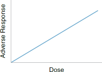
Some causal agents do not exhibit a linear dose–response relationship. For example, some agents may not cause disease until the exposure exceeds a certain threshold dose. Figure 10 depicts a dose–response relationship with a threshold, with a linear dose–response relationship for doses above the threshold.

There may be a no–effect threshold dose for some toxic substances, reflecting, for example, defense mechanisms and repair processes.235 However, for
234. Another dose–response relationship that may be of interest to researchers is the relationship of the severity of disease with increasing dose.
235. The idea that the “dose makes the poison” is a central tenet of toxicology, attributed to Paracelsus in the sixteenth century. See Eaton et al., supra note 60, “Introduction” section, in this
others such as carcinogens, it is commonly assumed that no threshold dose exists on a group basis.236 It is unlikely that researchers will find good evidence to support or refute the threshold–dose hypothesis because of the inability of epidemiology or animal toxicology to ascertain the effects of very small doses.237
Even if the incidence of disease increases with increasing dose, that dose–response relationship may not be linear. Supra-linear responses reflect a response that increases with increasing dose, but for which the rate of increase is smaller at higher doses than at lower doses, as depicted in Figure 11.238 Sub-linear responses reflect a response that increases with increasing dose, but for which the rate of increase is larger at higher doses than at lower doses, as depicted in Figure 12.239 Particularly for low-dose exposures, the shape of the dose–response curve—whether linear or curvilinear (and if the latter, the shape of the curve)—is a matter of hypothesis and speculation.240
manual. This dictum does not mean that any agent is capable of causing any disease if an individual is exposed to a sufficient dose. Rather, it reflects only the idea that there is a safe dose below which an agent does not cause any toxic effect. See Philip Wexler & Antoinette N. Hayes, The Evolving Journey of Toxicology: A Historical Glimpse, in Casarett and Doull’s Toxicology: The Basic Science of Poisons 3 (Curtis D. Klaassen ed., 9th ed. 2019); see also Alder v. Bayer Corp., AGFA Division, 61 P.3d 1068, 1088 (Utah 2002) (illustrating misunderstanding of the concept that “the dose makes the poison”). Toxic agents tend to cause specific harmful effects, an idea that also originated with Parcelsus. See section titled “Specificity of the Association” below.
236. See, e.g., Edward J. Calabrese et al., Ethical Challenges of the Linear Non-Threshold (LNT) Cancer Risk Assessment Revolution: History, Insights, and Lessons To Be Learned, 2022 Sci. Total Env’t 832, https://doi.org/10.1016/j.scitotenv.2022.155054; Bernd Kaina et al., Do Carcinogens Have a Threshold Dose? The Pros and Cons, in Regulatory Toxicology 397 (Franz-Xaver Reichl & Michael Schwenk eds., 2014). See also Irving J. Selikoff, Disability Compensation for Asbestos-Associated Disease in the United States: Report to the U.S. Department of Labor 181–220 (1981); Ferebee v. Chevron Chem. Co., 736 F.2d 1529, 1536 (D.C. Cir. 1984) (dose–response relationship for low doses is “one of the most sharply contested questions currently being debated in the medical community”); In re TMI Litig. Consol. Proc., 927 F. Supp. 834, 844–45 (M.D. Pa. 1996) (discussing low-dose extrapolation and the possibility of no-effect doses for radiation exposure and cancer).
237. Cf. Arnold L. Brown, The Meaning of Risk Assessment, 37 Oncology 302, 303 (1980); see also Advisory Comm. on Childhood Lead Poisoning Prevention, Ctrs. for Disease Control & Prevention, Low Level Lead Exposure Harms Children: A Renewed Call for Primary Prevention 7 (2012) (“new studies and re-interpretation of past studies have demonstrated that it is not possible to determine a threshold below which [blood lead level] is not inversely related to IQ”), https://stacks.cdc.gov/view/cdc/11859.
238. A supra-linear dose–response curve reveals a greater rate of response to increasing dose than would exist if the response rate were linear. A linear curve for the same dose and endpoint, see supra Figure 9, would be below the supra-linear curve depicted in Figure 11.
239. In contrast to a supra-linear curve, the responses in a sub-linear dose–response curve are lower than would exist if the response were linear. A linear curve for the same dose and endpoint, see supra Figure 9, would be above the sub-linear curve depicted in Figure 12.
240. See Allen v. United States, 588 F. Supp. 247, 419–24 (D. Utah 1984) (describing uncertainties about dose–response relationship at low levels of radiation exposure), rev’d on other grounds, 816 F.2d 1417 (10th Cir. 1987); In re Bextra & Celebrex Mktg. Sales Pracs. & Prod. Liab. Litig., 524 F. Supp. 2d 1166, 1180 (N.D. Cal. 2007) (criticizing expert for “primitive” extrapolation of
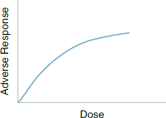
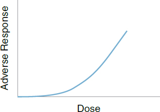
Finally, some agents may have a greater adverse effect on health outcomes at lower doses than at higher doses. Figure 13 depicts such a non-monotonic dose–response curve.241
Evidence for non-monotonic dose response has been presented for chemicals that affect hormones (termed endocrine disruptors) as well as for essential nutrients. In such cases, an association may be observed at lower doses and perhaps not at moderate or high doses. For example, while there is a range of manganese intake that contributes to normal child development, low manganese intake could impair normal bone formation, reproduction, and immune response;242 conversely, high exposure of pregnant women to manganese in
risk based on assumption of linear relationship of risk to dose); Troyen A. Brennan & Robert F. Carter, Legal and Scientific Probability of Causation for Cancer and Other Environmental Disease in Individuals, 10 J. Health Pol’y & L. 33, 43–44 (1985).
241. A non-monotonic effect is one in which the relationship between the response of the dependent variable does not continually proceed in the same direction as the independent variable, as shown in the dose–response curve in Figure 13.
242. See Longman Li & Xiaobo Yang, The Essential Element Manganese, Oxidative Stress, and Metabolic Diseases: Links and Interactions, Oxidative Med. Cell Longevity, Apr. 5, 2018, https://doi.org/10.1155/2018/7580707; Food & Nutrition Bd., Inst. Med., Dietary Reference Intakes for
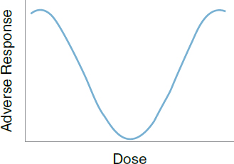
drinking water may impair cognition among their children.243 Thus, a dose–response relationship is supportive, but not essential, evidence that the relationship between an agent and disease is causal.244
Replication of the Findings
Rarely, if ever, does a single study persuasively demonstrate a cause–effect relationship.245 It is important that a study be repeated in different populations and by different investigators before a causal relationship is accepted by epidemiologists and other scientists.246
Vitamin A, Vitamin K, Arsenic, Boron, Chromium, Copper, Iodine, Iron, Manganese, Molybdenum, Nickel, Silicon, Vanadium, and Zinc (2001); Judy L. Aschner & Michael Aschner, Nutritional Aspects of Manganese Homeostasis, 26 Molecular Aspects Med. 353 (2005), https://doi.org/10.1016/j.mam.2005.07.003; Pan Chen et al., Manganese Metabolism in Humans, 23 Frontiers BioscienceLandmark 1655 (2018), https://doi.org/10.2741/4665.
243. See Kaitlin Vollet, Manganese Exposure and Cognition Across the Lifespan: Contemporary Review and Argument for Biphasic Dose–Response Health Effects, 3 Current Env’t Health Reps. 392 (2016), https://doi.org/10.1007/s40572-016-0108-x.
244. Evidence of a dose–response relationship as bearing on whether an inference of general causation is justified is analytically distinct from determining whether evidence of the dose to which a plaintiff was exposed is required in order to establish specific causation. On the latter matter, see section titled “Specific Causation” below; Restatement (Third) of Torts: Liability for Physical and Emotional Harm § 28 cmt. c(2) & rptrs. note (2010).
245. In Kehm v. Procter & Gamble Co., 580 F. Supp. 890, 901 (N.D. Iowa 1982), aff’d, 724 F.2d 613 (8th Cir. 1983), the court remarked on the persuasive power of multiple independent studies, each of which reached the same finding of an association between toxic shock syndrome and tampon use.
246. See Celentano & Szklo, supra note 37, at 277 (“Replication of findings is particularly important in epidemiology.”); In re Mirena IUS Levonorgestrel-Related Prods. Liab. Litig. (No. II), 341 F. Supp. 3d 213, 250 (S.D.N.Y. 2018) (citing the third edition of this reference guide), aff’d, 982 F.3d 113 (2d Cir. 2020). But see Smith v. Wyeth-Ayerst Labs. Co., 278 F. Supp. 2d 684, 710 n.55 (W.D.N.C. 2003) (observing that replication is difficult to establish when there is only one study that has been performed at the time of trial).
The importance of replicating research findings permeates most fields of science. In epidemiology, research, if repeated, often is repeated in different populations. Consistency of the findings of multiple investigations is an important factor in making a judgment about causation. Different studies that examine the same exposure–disease relationship generally should yield qualitatively similar, but likely not quantitatively identical, results.247 However, it is important to keep in mind that relations between exposures and outcomes may actually differ between populations because of differences in other factors (e.g., genetics, sociodemographic characteristics, nutrition).
Biological Plausibility
Biological plausibility is not an easy criterion to use and depends upon existing knowledge about the mechanisms by which the disease develops. When biological plausibility exists, it lends credence to an inference of causality.248 For example, the conclusion that high cholesterol is a cause of coronary heart disease is made more plausible because cholesterol is found in atherosclerotic plaques.249 However, observations have been made in epidemiologic studies that were not
247. See Valentin Amrhein et al., Inferential Statistics as Descriptive Statistics: There Is No Replication Crisis if We Don’t Expect Replication, 73 Am. Statistician 262 (2019), https://doi.org/10.1080/00031305.2018.1543137.
248. A number of courts have adverted to this criterion in the course of their discussions of causation in toxic substances cases. E.g., In re Phenylpropanolamine (PPA) Prods. Liab. Litig., 289 F. Supp. 2d 1230, 1247–48 (W.D. Wash. 2003); Cook v. United States, 545 F. Supp. 306, 314–15 (N.D. Cal. 1982) (discussing biological implausibility of a two-peak increase of disease when plotted against time); Landrigan v. Celotex Corp., 605 A.2d 1079, 1085–86 (N.J. 1992) (discussing the existence vel non of biological plausibility); see also Eaton et al., supra note 60, “Demonstrating an Association Between Exposure and Risk of Disease.”
249. High LDL cholesterol levels are associated with higher rates of coronary heart disease. The physical presence of cholesterol in plaques found in blood vessels lends credence—biological plausibility—to the idea that this association is causal. The causal relation has been confirmed by randomized clinical trials of statin drugs, which reduce blood levels of LDL cholesterol and have a protective effect against heart disease.
Epidemiologists have also used another approach to help rule out the possibility that the association resulted from the effects of some unknown confounder (a factor causing both high LDL cholesterol and coronary heart disease) or even the possibility that coronary heart disease causes LDL cholesterol to collect in plaques (i.e., so-called reverse causation). This approach relies on genetic variability to provide information about the causal role of cholesterol levels.
Some people have genetic variations that affect their metabolism of fats and reduce their LDL cholesterol levels. People with these cholesterol-lowering genes have reduced risk of coronary heart disease. The observation that an inherited genetic variation is associated with both lower LDL cholesterol levels and reduced risk of coronary heart disease strongly supports the inference that cholesterol levels affect the disease risk rather than heart disease causing cholesterol or confounding. Because the presence or absence of coronary heart disease does not affect an individual’s inherited genes, there is no possibility of reverse causation. Because some unknown factor does not alter both
biologically plausible at the time but that were subsequently shown to be correct.250 When an observation is inconsistent with current biological knowledge, it should not be discarded, but the observation should be confirmed before it is given credence. The salience of this factor varies depending on the extent of scientific knowledge about the toxicology as well as cellular and subcellular mechanisms through which the disease process works. The mechanisms of some diseases are understood quite well based on evidence, including from toxicologic research, whereas other mechanism explanations are merely hypothesized—although hypotheses are sometimes accepted under this factor.251
a person’s inherited genes and a person’s coronary heart disease risk, the possibility of confounding is greatly reduced (see section titled “Effect Modification” above).
This epidemiologic method—known as Mendelian randomization (named after Gregor Mendel, the pioneering researcher of the laws of heredity)—uses genetic variation (in the example, the cholesterol-lowering variant) as a proxy for an exposure of interest (in the example, LDL cholesterol levels), to help clarify whether the exposure is causally associated with a health outcome of interest (in the example, coronary heart disease). As vast genomic datasets are increasingly available, the number of studies applying Mendelian randomization is increasing rapidly.
Mendelian randomization can be applied when genetic variations are associated with the exposure of interest and certain other assumptions are satisfied. It might seem implausible that a genetic variation is associated with the likelihood that someone is exposed to a potentially toxic substance. But genetic variation could affect how a person metabolizes a substance, which in turn could affect the substance’s toxicity in that person. In such a situation, Mendelian randomization could be useful for the causal issues discussed in this reference guide; we thus provide this brief introduction to the methodology. As of the date of publication of this reference guide, however, Mendelian randomization has not been prominent in research on the types of causal issues addressed here and has not figured at all in court opinions concerning those issues. For short introductions to the methodology, see Gemma Sharp, Introduction to Mendelian Randomization, youtube.com/watch?v=isMZhasFc4M (Mar. 10, 2020) (last visited November 13, 2024); Connor A. Emdin et al., Mendelian Randomization, 318 JAMA 1925 (2017), https://doi.org/10.1001/jama.2017.17219. For a more mathematical introduction, see E. Sanderson et al., Mendelian Randomization, 2 Nature Rev. Methods Primers [6] (2022), https://doi.org/10.1038/s43586-021-00092-5.
250. For example, Sir Norman Gregg connected German measles in pregnant women with congenital cataracts before there was understanding of the role of viruses as teratogens. See Celentano & Szklo, supra note 37, at 277; N. McAllister Gregg, Congenital Cataract Following German Measles in the Mother, 107 Epidemiology & Infection iii (1991), https://doi.org/10.1017/s0950268800048627.
251. See Douglas L. Weed & Stephen D. Hursting, Biologic Plausibility in Causal Inference: Current Methods and Practice, 147 Am. J. Epidemiology 415 (1998), https://doi.org/10.1093/oxfordjournals.aje.a009466 (examining use of this criterion in contemporary epidemiologic research and distinguishing between alternative explanations of what constitutes biological plausibility, ranging from mere hypotheses to “sufficient evidence to show how the factor influences a known disease mechanism”); David A. Savitz, Epidemiology and Biological Plausibility in Assessing Causality, 5 Env’t Epidemiology e177 (2021), https://doi.org/10.1097/EE9.0000000000000177. For a discussion of the role of mechanistic research in toxicology, see Eaton et al., supra note 60, “Toxicological Processes and Target Organ Toxicity.”
Consideration of Alternative Explanations
This consideration refers to the possibility that an observed association is caused by something other than the exposure under study. The importance of considering the possibility of bias and confounding and ruling out those possibilities is discussed above.252
Cessation of Exposure
If an agent is a cause of a disease, then one would expect that cessation of exposure to that agent ordinarily would reduce the risk of the disease.253 This has been the case, for example, with cigarette smoking and lung cancer. In many situations, however, relevant data are simply not available regarding the possible effects of ending the exposure. But when such data are available, and eliminating exposure reduces the incidence of disease, this factor strongly supports a causal relationship.
Specificity of the Association
An association exhibits specificity if the exposure is associated only with a single disease or type of disease. This criterion reflects the fact that although an agent causes one disease, it does not necessarily cause other diseases.254 This
252. See sections titled “Biases” and “Effect Modification” above.
253. In his speech, Hill labeled this consideration “Experiment” because, as compared to other types of observational studies, the ability to observe what happens when an exposure ceases is more closely akin to a controlled experiment.
254. See, e.g., Nelson v. Am. Sterilizer Co., 566 N.W.2d 671, 676–77 (Mich. Ct. App. 1997) (affirming dismissal of plaintiff’s claims that chemical exposure caused her liver disorder, but recognizing that evidence supported claims for neuropathy and other illnesses); Sanderson v. Int’l Flavors & Fragrances, Inc., 950 F. Supp. 981, 996–98 (C.D. Cal. 1996); see also Taylor v. Airco, Inc., 494 F. Supp. 2d 21, 27 (D. Mass. 2007) (holding that plaintiff’s expert could testify to causal relationship between vinyl chloride and one type of liver cancer for which there was only modest support given strong causal evidence for vinyl chloride and another type of liver cancer).
When a party claims that evidence of a causal relationship between an agent and one disease is relevant to whether the agent caused another disease, courts have required the party to show that the mechanisms involved in development of the disease are similar. For example, in Milward v. Acuity Specialty Products, 639 F.3d 11, 19–20 (1st Cir. 2011), the court accepted the plaintiff’s expert’s testimony that benzene caused a rare form of leukemia based on studies supporting the proposition that benzene was a cause of the general form of leukemia and testimony about the common causal mechanism for all types of leukemia. Accord In re Bextra & Celebrex Mktg. Sales Pracs. & Prod. Liab. Litig., 524 F. Supp. 2d 1166, 1183 (N.D. Cal. 2007); Magistrini v. One-Hour Martinizing Dry Cleaning, 180 F. Supp. 2d 584, 603 (D.N.J. 2002).
consideration is highly debatable. Evidence amassed since the publication of Hill’s paper runs contrary to this. For example, cigarette manufacturers have long claimed that because cigarettes have been linked to multiple adverse health outcomes including lung cancer, emphysema, bladder cancer, heart disease, pancreatic cancer, and other conditions, there is no specificity and the relationships are not causal. There is, however, at least one good reason why inferences about the health consequences of tobacco do not require specificity: Because tobacco and cigarette smoke are not in fact single agents but consist of numerous harmful agents, smoking represents exposure to multiple agents, with multiple potential effects. However, even a single chemical can increase risk for multiple disease endpoints, e.g., multiple cancers.255 For example, asbestos causes both lung cancer and mesothelioma.
Consistency with Other Relevant Knowledge
In addressing the causal relationship of lung cancer to cigarette smoking, researchers examined trends over time for lung cancer and for cigarette sales in the United States. A marked increase in lung-cancer death rates in men was observed with a time lag reflecting the latency period for lung cancer, which appeared to follow the increase in sales of cigarettes. Had the increase in lung-cancer deaths followed a decrease in cigarette sales, it might have given researchers pause. It would not have precluded a causal inference, but the inconsistency of the trends in cigarette sales and lung-cancer mortality would have had to be explained.
Background Rate of Disease
The background rate of disease is neither a Hill/Gordis factor256 nor a consideration involved in determining whether an association should be judged as causal. Still, some courts have stated that, independent of epidemiologic studies, the background rate of the disease at issue must be identified and known by an
255. See, e.g., Dario Consonni et al., Mortality and Cancer Incidence in a Population Exposed to TCDD After the Seveso, Italy, Accident (1976-2013), 81 Occup. Env’t Med. 349 (2024) (describing association of exposure with various cancers and other illnesses after an accidental release of dioxin, depending on geographic location relative to the accident, gender, and time after the accident); Marcella Warner et al., Dioxin Exposure and Cancer Risk in the Seveso Women’s Health Study, 119 Env’t Health Persps. 1700, 1703 (2011) (reporting “a statistically significant, dose–related increased risk in overall cancer incidence associated with” levels of dioxin in blood).
256. This refers to the considerations for assessing the causal significance of an association first described by Sir Austin Bradford Hill as modified by Leon Gordis. See supra note 218.
expert testifying to general causation.257 This is incorrect and fails to appreciate epidemiologic methodology. Epidemiologists examine the difference in rates of disease between the exposed and unexposed groups in a study.258 In a well-designed epidemiologic study, the “background” rate—the likelihood of disease even absent exposure—will be reflected in the rate of disease in the unexposed group.259 The magnitude of the background rate is unimportant for determining if that rate is different from the rate in the exposed group. To put the point slightly differently, whether the background rate is very low, moderate, or relatively high does not affect the researcher’s assessment of the data’s probative value for determining general causation.260
Methods for Synthesizing or Combining the Results of Multiple Studies
The scientific record often includes a number of epidemiologic studies examining a similar exposure and outcome. Often those studies will have different
257. See In re Deepwater Horizon Belo Cases, No. 3:19CV963-MCR-HTC, 2022 WL 17721595, at *5 (N.D. Fla. Dec. 15, 2022) (“Thus, a failure to identify or describe the background risk of a disease is a ‘serious methodological deficiency’ and ‘substantial weakness’ in an expert’s general causation opinion.”) (quoting Chapman v. Procter & Gamble Distrib., LLC, 766 F.3d 1296, 1307 (11th Cir. 2014)); In re Abilify (Aripiprazole) Prods. Liab. Litig., 299 F. Supp. 3d 1291, 1308 (N.D. Fla. 2018); Jones v. Novartis Pharms. Corp., 235 F. Supp. 3d 1244, 1280 (N.D. Ala. 2017) (“A failure to assess or identify the background risk of a disease is a ‘serious methodological deficiency’ because, ‘[w]ithout a baseline, any incidence may be coincidence.’”) (quoting Chapman v. Procter & Gamble Distrib., LLC, 766 F.3d 1296, 1307-08 (11th Cir. 2014)), aff’d in part, 720 F. App’x 1006 (11th Cir. 2018).
258. See section titled “Relative Risk” above. Alternatively, in a case-control design, epidemiologists examine the difference in the odds of exposure among groups with and without the disease. See section titled “Odds Ratio” above.
259. This is not to say that the background rate of disease is entirely unimportant to epidemiologists. If a disease is very rare, it may be difficult to conduct a study with enough subjects to generate statistically meaningful results, even if an exposure actually causes the disease. The background rate of disease also may play an important role in public health decision-making, as it can address the relative benefit of an intervention that reduces that rate of disease.
260. Some courts have implied that the presence of a relatively high background rate of a disease itself undermines an inference of general causation. To see why this is incorrect, imagine a disease that afflicts as many as 20% of the general population, but that—as revealed by a well-designed epidemiologic study—afflicts 100% of people exposed to a particular agent. In this example, the relative risk would be 5.0. We likely would have no trouble making the inference that the agent causes at least some cases of disease among those exposed, assuming that the relevant considerations epidemiologists take into account, see supra text accompanying notes 218–54, support that inference. The same would be equally true with an extremely low background rate of disease that was five times greater in the exposed group.
results; even with well-conducted studies, we should expect to find variation in the results.261 Some may find an association while others may not, or studies may report associations, but of different magnitude.262 Different studies may also be conducted in populations with different characteristics, apply different statistical techniques, measure exposure or the outcome differently, or control for different confounders, among other things, which may explain the different results. There are two main types of data-synthesis methodologies available when multiple studies address an issue of scientific interest: 1) systematic review263 and 2) meta-analysis.264 The two are similar in that they do not directly investigate the question of interest by gathering and analyzing primary data, but instead synthesize studies that have been previously performed. Systematic reviews265 are not quantitative; meta-analyses provide a quantitative summary of data gathered by multiple prior studies. Both are important because science is a cumulative process and all relevant prior work should be considered when addressing a scientific issue. Systematic reviews have been described as “a review of evidence relevant to a clearly formulated question that uses systematic and explicit methods to identify, select and critically appraise relevant research, and to collect and analyze data from the studies that are included within the review.”266
In view of the fact that studies may disagree and that studies may be based on a small number of individuals and lack the statistical power needed for firmer conclusions, the technique of meta-analysis was developed.267 Meta-analysis is a
261. See Valentin Amrhein et al., Inferential Statistics as Descriptive Statistics: There Is No Replication Crisis if We Don’t Expect Replication, 73 Am. Statistician 262 (2019), https://doi.org/10.1080/00031305.2018.1543137.
262. See, e.g., Zandi v. Wyeth a/k/a Wyeth, Inc., No. 27-CV-06-6744, 2007 WL 3224242 (Minn. Dist. Ct. Oct. 15, 2007) (plaintiff’s expert cited 40 studies in support of a causal relationship between hormone therapy and breast cancer; many studies found different magnitudes of increased risk).
263. See generally Cochrane Handbook for Systematic Reviews of Interventions (Julian P.T. Higgins et al. eds., 2d ed. 2019). A set of guidelines, Preferred Reporting Items for Systematic Reviews and Meta-Analysis (PRISMA), is used for systematic reviews to provide consistency and transparency and to improve the reliability of the reviews. See Matthew J. Page et al., The PRISMA 2020 Statement: An Updated Guideline for Reporting Systematic Reviews, 372 Brit. Med. J. n.71 (2021), https://doi.org/10.1136/bmj.n71.
264. See Savitz & Wellenius, supra note 222, at 185–98.
265. See generally Guy Paré & Spyros Kitsiou, Methods for Literature Reviews, in Handbook of eHealth Evaluation: An Evidence-Based Approach (F. Lau & C. Kuziemsky eds., 2017), https://perma.cc/RBF7-7FXE.
266. Env’t Evidence, Systematic Review, Collaboration for Env’t Evidence, https://perma.cc/9RHX-KB2K.
267. See In re Paoli R.R. Yard PCB Litig., 916 F.2d 829, 856 (3d Cir. 1990); In re Viagra (Sildenafil Citrate) & Cialis (Tadalafil) Prods. Liab. Litig., 424 F. Supp. 3d 781, 787 (N.D. Cal. 2020) (“Meta-analysis has the advantage of pooling more data so that the results are less likely to be misleading solely due to chance.”). Thus, contrary to the suggestion by at least one court, multiple studies with small numbers of subjects may be pooled to reduce the possibility of sampling error. See In re Joint E. & S. Dist. Asbestos Litig., 827 F. Supp. 1014, 1042 (S.D.N.Y. 1993) (“[N]o matter
method of pooling study results to arrive at a single measure of association to represent the totality of the studies reviewed.268 It is a way of systematizing the time-honored approach of reviewing the literature, which is characteristic of science, and placing it in a standardized framework with quantitative methods for estimating associations. In a meta-analysis, studies are given different weights in proportion to the sizes of their study populations and other characteristics.269
Meta-analysis is most useful when employed in pooling randomized experimental trials, because in that circumstance the studies included in the meta-analysis share an important methodologic characteristic, namely the randomized assignment of subjects to different exposure groups.270 Meta-analysis applied to observational studies is also useful but is more challenging.271 Studies may vary in the methods employed (e.g., research design and statistical approaches) as well as in the extent to which they are affected by and may have adjusted or corrected for confounding, selection bias, and measurement error. Such differences raise questions about the appropriateness of combining studies’ results. The production of a single estimate of association, sometimes with a narrow confidence interval, may thus provide a false sense of security. Meta-analyses should be evaluated as carefully as one would evaluate the overall literature to draw a conclusion about the likelihood that an exposure causes a disease.272 For
how many studies yield a positive but statistically insignificant SMR for colorectal cancer, the results remain statistically insignificant. Just as adding a series of zeros together yields yet another zero as the product, adding a series of positive but statistically insignificant SMRs together does not produce a statistically significant pattern.”), rev’d, 52 F.3d 1124 (2d Cir. 1995).
268. For a nontechnical explanation of meta-analysis, along with case studies of a variety of scientific areas in which it has been employed, see Morton Hunt, How Science Takes Stock: The Story of Meta-Analysis (1997).
269. Petitti, supra note 121.
270. On rare occasions, meta-analyses of both clinical and observational studies are available. See, e.g., In re Bextra & Celebrex Mktg. Sales Pracs. & Prod. Liab. Litig., 524 F. Supp. 2d 1166, 1175 (N.D. Cal. 2007) (referring to clinical and observational meta-analyses of a low dose of a drug; both analyses failed to find any effect).
271. See Jesse A. Berlin et al., The Use of Meta-Analysis in Pharmacoepidemiology, in Pharmacoepidemiology, at 897, 899–901 (Brian L. Strom et al. eds., 6th ed. 2020); Donna F. Stroup et al., Meta-Analysis of Observational Studies in Epidemiology: A Proposal for Reporting, 283 JAMA 2008, 2009 (2000), https://doi.org/10.1001/jama.283.15.2008; Zachary B. Gerbarg & Ralph I. Horwitz, Resolving Conflicting Clinical Trials: Guidelines for Meta-Analysis, 41 J. Clinical Epidemiology 503 (1988), https://doi.org/10.1016/0895-4356(88)90053-4. See also Deutsch v. Novartis Pharm. Corp., 768 F. Supp. 2d 420, 451–52 (E.D.N.Y. 2011) (rejecting defendants’ claim that meta-analysis is sufficiently reliable to support an expert opinion only if the meta-analysis is applied to clinical trials).
272. Courts have recognized that a properly performed meta-analysis can provide a basis for admissible expert testimony. In Cooper v. Takeda Pharms. Am., Inc., 191 Cal. Rptr. 3d 67, 95 (Ct. App. 2015), the court reinstated a jury verdict for the plaintiffs, observing that in striking plaintiffs’ experts’ testimony after trial, “the trial court’s piecemeal rejection of individual studies
instance, it is essential to ensure that the meta-analysis is well conducted. A well-conducted meta-analysis appropriately considers 1) the quality of the included studies, 2) whether publication bias (the greater probability of publication of significant findings) is likely to be present, 3) if unpublished studies should be sought and included, 4) whether criteria for including and excluding studies are appropriate, 5) whether appropriate subgroup analyses were conducted, and 6) whether results are exceedingly heterogeneous, and if so, whether the sources of heterogeneity (such as whether the effect of an exposure is truly different in populations with different characteristics) have been appropriately investigated.273
Specific Causation
Epidemiology is concerned with the incidence of disease in populations, and epidemiologic studies do not address the question of the cause of an individual’s
was inappropriate and ignored the testimony by [plaintiffs’ experts] that the results of the individual studies considered as a whole, including in the meta-analyses, was what really persuaded them that Actos causes bladder cancer.” Similarly reflecting the value of meta-analysis, in In re Bextra & Celebrex Mktg. Sales Pracs. & Prod. Liab. Litig., 524 F. Supp. 2d 1166 (N.D. Cal. 2007), the court relied on several meta-analyses of Celebrex at a 200-mg dose to conclude that the plaintiffs’ experts who proposed to testify to toxicity at that dosage failed to meet the requirements of Daubert. The court criticized those experts for the wholesale rejection of meta-analyses of observational studies. And, in In re Paoli Railroad Yard PCB Litig., 916 F.2d 829, 856–57 (3d Cir. 1990), the court overturned the district court’s exclusion of a report that used meta-analysis, observing that meta-analysis is a regularly used scientific technique. But the Third Circuit recognized that the technique might be poorly performed and required the district court to reconsider the validity of the expert’s work in performing the meta-analysis. See also In re Zoloft (Sertraline Hydrochloride) Prod. Liab. Litig., 858 F.3d 787, 796 (3d Cir. 2017) (affirming exclusion of expert testimony that involved meta-analyses because, even assuming that meta-analysis is a reliable technique, the expert did not “reliably apply the ‘technique’ to the body of evidence . . .”); Carl v. Johnson & Johnson, 237 A.3d 308 (N.J. Super. Ct. App. Div. 2020) (reversing exclusion of plaintiffs’ experts’ testimony and holding that the experts, who relied heavily on meta-analyses to support their opinions, “adhered to methodologies generally followed by experts in the field and relied upon studies and information generally considered an acceptable basis for inclusion in the formulation of expert opinions”).
273. See Mathew J. Page et al., The PRISMA 2020 Statement: an Updated Guideline for Reporting Systematic Reviews, 134 J. Clinical Epidemiology 178, 186 (2021), https://doi.org/10.1136/bmj.n71 (consensus statement describing update to a checklist of items to be included for “more transparent, complete, and accurate reporting of systematic reviews, thus facilitating evidence based decision making”); Stroup et al., supra note 271, at 2009 (consensus statement providing checklist of items to report in a meta-analysis based on a systematic review of published meta-analyses); Monika Mueller et al., Methods to Systematically Review and Meta-Analyse Observational Studies: A Systematic Scoping Review of Recommendations, 18 BMC Med. Rsch. Methodology 44 (2018), https://doi.org/10.1186/s12874-018-0495-9 (summarizing recommendations for conducting meta-analyses of observational studies).
disease.274 This question, often referred to as specific causation, is beyond the domain of the science of epidemiology.275
Epidemiology has its limits at the point where an inference is made that the relationship between an agent and a disease is causal (general causation) and where the magnitude of excess risk attributed to the agent has been determined; that is, epidemiologists investigate whether an agent can cause a disease, not whether an agent did cause a specific plaintiff’s disease.276
Nevertheless, the specific causation issue is a necessary legal element in a toxic tort case. The plaintiff must establish not only that the defendant’s agent is capable of causing disease generally, but also that it caused the plaintiff’s disease specifically.277 Thus, numerous cases have confronted the question of what is acceptable proof of specific causation and the role that epidemiologic evidence plays in answering that question.278 But this question is not addressed by
274. See DeLuca v. Merrell Dow Pharms., Inc., 911 F.2d 941, 945 & n.6 (3d Cir. 1990) (“Epidemiological studies do not provide direct evidence that a particular plaintiff was injured by exposure to a substance.”); Rhyne v. U.S. Steel Corp., 474 F. Supp. 3d 733, 750 (W.D.N.C. 2020) (“epidemiology focuses on the issue of general causation, not specific causation”); In re E. I. du Pont de Nemours & Co. C-8 Pers. Inj. Litig., No. 2:18-CV-00136, 2019 WL 6894069, at *6 (S.D. Ohio Dec. 18, 2019) (explaining that epidemiology focuses on general causation as opposed to specific causation (citing the third edition of this reference guide)); Michael Dore, A Commentary on the Use of Epidemiological Evidence in Demonstrating Cause-in-Fact, 7 Harv. Env’t L. Rev. 429, 436 (1983); Khristine L. Hall & Ellen K. Silbergeld, Reappraising Epidemiology: A Response to Mr. Dore, 7 Harv. Env’t L. Rev. 441, 445 (1983).
There are, however, some diseases that do not occur without exposure to a given toxic agent. This is the same as saying that the toxic agent is a necessary cause for the disease, and the disease is sometimes referred to as a signature disease (also, the agent is pathognomonic) because the existence of the disease necessarily implies the causal role of the agent. Two examples are asbestosis, which is a signature disease for asbestos, and vaginal adenocarcinoma (in young adult women), which is a signature disease for in utero DES exposure. See Kenneth S. Abraham & Richard A. Merrill, Scientific Uncertainty in the Courts, in Issues Sci. & Tech. 93, 101 (1986).
275. See Jones v. Novartis Pharms. Corp., 235 F. Supp. 3d 1244, 1252 (N.D. Ala. 2017) (“No scientific methodology exists for assessing specific causation for an individual based on group studies.”), aff’d in part, Jones v. Novartis Pharms. Co., 720 F. App’x 1006 (11th Cir. 2018).
276. See In re E. I. du Pont de Nemours & Co. C-8 Pers. Inj. Litig., No. 2:18-CV-00136, 2019 WL 6894069, at *6 (S.D. Ohio Dec. 18, 2019) (quoting the third edition of this reference guide).
277. See, e.g., Adkisson v. Jacobs Eng’g Grp., Inc., 342 F. Supp. 3d 791, 798 (E.D. Tenn. 2018) (explaining the difference between general causation and specific causation and observing the distinction is “well-accepted in federal courts”). Specific-causation evidence only matters when general causation has been established. See Williams v. Mosaic Fertilizer, No. 8:14-CV-1748-T-35MAP, 2016 WL 7175657, at *11 (M.D. Fla. June 24, 2016) (“Without an adequate basis for establishing general causation, Dr. Mink’s specific causation opinions are irrelevant.”), aff’d, 889 F.3d 1239 (11th Cir. 2018).
278. In many instances, causation can be established without epidemiologic evidence. When the mechanism of causation is well understood, the causal relationship is well established, or the timing between cause and effect is close, scientific evidence of causation may not be required. This is frequently the situation when the plaintiff suffers traumatic injury rather than disease. This
epidemiology.279 It is instead a legal question—one with which numerous courts have grappled.280 The remainder of this section is predominantly an explanation of judicial opinions and the reasoning courts have used in applying risk estimates from epidemiology to address the issue of specific causation in individual cases.
Before proceeding, one last caveat is in order. This section assumes that epidemiologic evidence has been used as proof of causation for a given plaintiff. The discussion does not address whether a plaintiff must or should use epidemiologic evidence to prove causation.281
section addresses only those situations in which causation is not evident, and scientific evidence is required.
279. Nevertheless, an epidemiologist may be helpful to the factfinder answering this question. Some courts have permitted epidemiologists, or those who use epidemiologic methods, to testify about specific causation. See Ambrosini v. Labarraque, 101 F.3d 129, 137–41 (D.C. Cir. 1996); Zuchowicz v. United States, 870 F. Supp. 15 (D. Conn. 1994); Landrigan v. Celotex Corp., 605 A.2d 1079, 1088–89 (N.J. 1992); Carl v. Johnson & Johnson, 237 A.3d 308, 338 (N.J. Super. App. Div. 2020). But see Rhyne v. U.S. Steel Corp., 474 F. Supp. 3d 733, 750 (W.D.N.C. 2020) (concluding epidemiologist was not qualified to testify to specific causation).
In general, courts seem more concerned with the basis of an expert’s opinion than with whether the expert is an epidemiologist or clinical physician. See Porter v. Whitehall, 9 F.3d 607, 614 (7th Cir. 1992) (“curb side” opinion from clinician not admissible); Burton v. R.J. Reynolds Tobacco Co., 181 F. Supp. 2d 1256, 1266–67 (D. Kan. 2002) (vascular surgeon permitted to testify to general causation over objection based on fact he was not an epidemiologist); Wade-Greaux v. Whitehall Labs., 874 F. Supp. 1441, 1469–72 (D.V.I.) (clinician’s multiple bases for opinion inadequate to support causation opinion), aff’d, 46 F.3d 1120 (3d Cir. 1994); Landrigan, 605 A.2d at 1083–89 (permitting both clinicians and epidemiologists to testify to specific causation provided the methodology used is sound); Trach v. Fellin, 817 A.2d 1102, 1118–19 (Pa. Super. Ct. 2003) (toxicologist and pathologist permitted to testify to specific causation).
280. See Restatement (Third) of Torts: Liability for Physical and Emotional Harm § 28 cmt. c(3) (2010) (“Scientists who conduct group studies do not examine specific causation in their research. No scientific methodology exists for assessing specific causation for an individual based on group studies. Nevertheless, courts have reasoned from the preponderance-of-the-evidence standard to determine the sufficiency of scientific evidence on specific causation when group-based studies are involved. . . .”).
281. See id. § 28 cmt. c(3) & rptrs. note (“most courts have appropriately declined to impose a threshold requirement that a plaintiff always must prove causation with epidemiologic evidence”); see also Westberry v. Gislaved Gummi AB, 178 F.2d 257 (4th Cir. 1999) (holding that expert’s testimony on causation was properly admitted where there was an acute response, a differential diagnosis that ruled out other known causes of disease, and the absence of epidemiologic or toxicologic studies and there were dechallenge/rechallenge tests conducted by expert that were consistent with exposure to defendant’s agent causing disease); Zuchowicz v. United States, 140 F.3d 381 (2d Cir. 1998); In re Testosterone Replacement Therapy Prods. Liab. Litig. Coordinated Pretrial Proc., No. 14 C 1748, 2017 WL 1833173, at *15 (N.D. Ill. May 8, 2017) (“Where the existing epidemiological research is limited or nonexistent, courts are more willing to allow expert testimony on causation that does not depend on epidemiological sources.”) (citing cases); In re Tylenol (Acetaminophen) Mktg., Sales Pracs. & Prods. Liab. Litig., No. 2:12-CV-07263, 2016 WL 3997046, at *7 (E.D. Pa. July 26, 2016) (rejecting defendant’s contention that because there were no epidemiologic studies available, plaintiff’s expert could not testify to causation of liver failure due to Tylenol use and explaining the reasons why such studies were unavailable for such a relationship).
Two legal issues arise with regard to the role of epidemiology in proving individual causation: admissibility and sufficiency of evidence to meet the burden of production. The first issue tends to receive less attention by the courts, because epidemiologic studies are rarely introduced independently into evidence,282 but nevertheless deserves mention: An epidemiologic study that is sufficiently rigorous to justify a conclusion that it is scientifically valid should be admissible,283 as it tends to make an issue in dispute more or less likely.284
Far more courts have confronted the role that epidemiology plays with regard to the sufficiency of the evidence and the burden of production.285 The civil burden of proof is described most often as requiring the factfinder to “believe that what is sought to be proved . . . is more likely true than not true.”286 The relative risk from epidemiologic studies can be adapted to this 50%-plus standard to yield a probability or likelihood that an agent caused an individual’s disease.287 But while the discussion below speaks in terms of the magnitude of
282. Most often, epidemiologic and other scientific studies are used by expert witnesses as the basis of their causal opinions and are not independently admitted into evidence.
283. See DeLuca v. Merrell Dow Pharms., Inc., 911 F.2d 941, 958 (3d Cir. 1990); cf. Kehm v. Procter & Gamble Co., 580 F. Supp. 890, 902 (N.D. Iowa 1982) (“These [epidemiologic] studies were highly probative on the issue of causation—they all concluded that an association between tampon use and menstrually related TSS [toxic shock syndrome] cases exists.”), aff’d, 724 F.2d 613 (8th Cir. 1984). In Ellis v. International Playtex, Inc., 745 F.2d 292, 303 (4th Cir. 1984), the court concluded that certain epidemiologic studies were admissible under an exception to the hearsay rule despite criticism of the methodology used in the studies. The court held that the claims of bias went to the studies’ weight rather than their admissibility.
284. Even if evidence is relevant, it may be excluded if its probative value is substantially outweighed by prejudice, confusion, or inefficiency. Fed. R. Evid. 403. In Daubert, 509 U.S. at 591, the Court invoked the concept of “fit,” which addresses the relationship of the basis for an expert’s scientific opinion to the facts of the case and the issues in dispute. In a toxic substance case in which cause in fact is disputed, an epidemiologic study of the same agent to which the plaintiff was exposed that examined the association with the same disease from which the plaintiff suffers would undoubtedly have sufficient “fit” to be a part of the basis of an expert’s opinion. The Court’s concept of “fit,” borrowed from United States v. Downing, 753 F.2d 1224, 1242 (3d Cir. 1985), appears equivalent to the more familiar evidentiary concept of probative value, albeit one requiring assessment of the scientific reasoning the expert used in drawing inferences from methodology or data to opinion.
285. We reiterate a point made at the outset of this section: This discussion of the use of a threshold relative risk for specific causation is not epidemiology or an inquiry an epidemiologist would undertake but an effort by courts and commentators to adapt the legal standard of proof to the available scientific evidence. See supra text accompanying notes 274–76.
286. Edward J. Devitt & Charles B. Blackmar, 2 Federal Jury Practice and Instruction § 71.13 (3d ed. 1977); see also United States v. Fatico, 458 F. Supp. 388, 403 (E.D.N.Y. 1978) (“Quantified, the preponderance standard would be 50%+ probable.”), aff’d, 603 F.2d 1053 (2d Cir. 1979).
287. An adherent of the frequentist school of statistics would resist this adaptation, which may explain why many epidemiologists and toxicologists also resist it. To use an epidemiologic study outcome to determine the probability of specific causation requires a shift from a frequentist approach, which involves sampling or frequency data from an empirical test, to a subjective probability about a discrete event. A frequentist might assert, after conducting a sampling test, that 60%
the relative risk or association found in a study, before an association or relative risk is used to make a statement about the probability of individual causation, the inferential judgment288 that the association is truly causal is required. “[A]n agent cannot be considered to cause the illness of a specific person unless it is recognized as a cause of that disease in general.”289 The following discussion should be read with this caveat in mind.290
Some courts have reasoned that when epidemiologic studies find that exposure to the agent causes an incidence in the exposed group more than twice the incidence in the unexposed group (i.e., a relative risk greater than 2.0), the probability that exposure to the agent caused a similarly situated individual’s disease is greater than 50%. These courts hold that when there is group-based evidence finding that exposure to an agent causes an incidence of disease in the exposed group that is more than twice the incidence in the unexposed group, the evidence is sufficient to satisfy the plaintiff’s burden of production and permit submission of specific causation to a jury. In such a case, the factfinder may find that it is more likely than not that the substance caused the particular plaintiff’s disease.291 Courts, thus, have permitted expert witnesses to testify to specific causation based on the logic of the effect of a doubling of the risk.292
of the balls in an opaque container are blue. The same frequentist would resist the statement, “The probability that a single ball removed from the box and hidden behind a screen is blue is 60%.” The ball is either blue or not, and no frequentist data would permit the latter statement. “[T]here is no logically rigorous definition of what a statement of probability means with reference to an individual instance. . . .” Lee Loevinger, On Logic and Sociology, 32 Jurimetrics J. 527, 530 (1992), https://doi.org/10.2307/1190721; see also Steve Gold, Causation in Toxic Torts: Burdens of Proof, Standards of Persuasion and Statistical Evidence, 96 Yale L. J. 376, 382–92 (1986). Subjective probabilities about unique events are employed by those using Bayesian methodology. See Kaye, supra note 115, at 54–62; Kaye & Stern, supra note 16, “What is Bayes’ Rule?”
288. This is described in the section titled “Effect Modification” above.
289. Cole, supra note 94, at 10,284.
290. We emphasize this point both because it is not intuitive and because some courts have failed to appreciate the difference between an association and a causal relationship. See, e.g., Forsyth v. Eli Lilly & Co., Civil No. 95-00185 ACK, 1998 U.S. Dist. LEXIS 541, at *26–*31 (D. Haw. Jan. 5, 1998). But see Berry v. CSX Transp., Inc., 709 So. 2d 552, 568 (Fla. Dist. Ct. App. 1998) (“From epidemiologic studies demonstrating an association, an epidemiologist may or may not infer that a causal relationship exists.”).
291. A similar means to address probabilities in individual cases is use of the attributable risk (or attributable fraction parameter). The attributable risk is that portion of the excess risk that can be attributed to an agent, above and beyond the background risk that is due to other causes. See section titled “Attributable Risk” above. Thus, when the relative risk is greater than 2.0, the attributable fraction exceeds 50%.
292. For a comprehensive, if dated, list of cases that support proof of causation based on group studies, see Restatement (Third) of Torts: Liability for Physical and Emotional Harm § 28 cmt. c(4) rptrs. note (2010). The Restatement catalogs those courts that require a relative risk in excess of 2.0 as a threshold for sufficient proof of specific causation and those courts that recognize that even a lower relative risk than that can support specific causation, as explained below. Despite considerable disagreement on whether a relative risk of 2.0 is required or merely a taking-off point for determining
While this reasoning has a certain logic as far as it goes, there are a number of significant assumptions that require explication. These are addressed below.
A Valid Study and Risk Estimate.
The propriety of this “doubling” reasoning depends on group studies identifying a genuine causal relationship and a reasonably reliable measure of the increased risk.293 This requires attention to the possibility of random error, bias, or confounding being the source of the association rather than a true causal relationship, as explained in the sections above titled “Sources of Error in Epidemiologic Studies” and “General Causation.”
Similarity of Study Participants and Plaintiff.
Only if the study participants and the plaintiff are similar with respect to relevant risk factors will a risk estimate from a study or studies be valid when applied to an individual.294 Thus, if those exposed in a study of the risk of lung cancer from smoking have smoked half a pack of cigarettes a day for 20 years, the degree of increased incidence of lung cancer among them cannot be extrapolated to someone who smoked two packs of cigarettes for 30 years, without strong assumptions about the dose–response relationship.295 This principle is also applicable to risk factors for competing causes. If all of the participants in a study are participating because they were identified as
the sufficiency of the evidence on specific causation, two commentators who surveyed the cases observed that “[t]here were no clear differences in outcomes as between federal and state courts.” Russellyn S. Carruth & Bernard D. Goldstein, Relative Risk Greater than Two in Proof of Causation in Toxic Tort Litigation, 41 Jurimetrics J. 195, 199 (2001), https://www.jstor.org/stable/29762698.
293. Indeed, one commentator contends that because epidemologic studies often are insufficiently precise to accurately measure small increases in risk, in general, studies that find a relative risk less than 2.0 should not be sufficient for causation. This concern is not with specific causation, but with general causation and the likelihood that an association less than 2.0 is noise rather than reflecting a true causal relationship. See Michael D. Green, The Future of Proportional Liability, in Exploring Tort Law (Stuart Madden ed., 2005); see also Robert F. Reynolds, The Use of Randomized Controlled Trials for Pharmacoepidemiology, in Pharmacoepidemilogy 792, 794 (Brian L. Strom ed., 4th ed. 2005) (cautioning that small relative risks in observational studies can be the product of confounding); Gary Taubes, Epidemiology Faces Its Limits, 269 Sci. 164 (1995) (explaining views of several epidemiologists about a threshold relative risk of 3.0 to seriously consider a causal relationship); N.E. Breslow & N.E. Day, Statistical Methods in Cancer Research, in The Analysis of Case-Control Studies 36 (IARC Pub. No. 32, 1980) (“[r]elative risks of less than 2.0 may readily reflect some unperceived bias or confounding factor”); David A. Freedman & Philip B. Stark, The Swine Flu Vaccine and Guillain-Barré Syndrome: A Case Study in Relative Risk and Specific Causation, 64 Law & Contemp. Probs. 49, 61 (2001), https://doi.org/10.1177/0193841X9902300603 (“If the relative risk is near 2.0, problems of bias and confounding in the underlying epidemiologic studies may be serious, perhaps intractable.”).
294. Council on Sci. Affs., Am. Med. Ass’n, Radioepidemiological Tables, 257 JAMA 806, 807 (1987) (“The basic premise of probability of causation is that individual risk can be determined from epidemiologic data for a representative population; however, the premise only holds if the individual is truly representative of the reference population.”).
295. Conversely, a risk estimate from a study that involved a greater exposure is not applicable to an individual exposed to a lower dose. See, e.g., In re Bextra & Celebrex Mktg. Sales Pracs. & Prod. Liab. Litig., 524 F. Supp. 2d 1166, 1175–76 (N.D. Cal. 2007) (relative risk found in studies of those who took twice the dose of others could not support an expert’s opinion of causation for the latter group); In re Bextra & Celebrex, No. 762000/2006, 2008 N.Y. Misc. LEXIS 720, at *29 (Sup.
having a family history of heart disease, the magnitude of risk found in a study of the effect of smoking on the risk of heart disease cannot validly be applied to an individual without such a family history.296
Similarly, if an individual has been differentially exposed to other risk factors from those in a study, the results of the study will not provide an accurate basis for the probability of causation for the individual.297 Consider a study of the effect of smoking on lung cancer among subjects who have no asbestos exposure. The relative risk of smoking in that study would not be applicable to an asbestos insulation worker.
More generally, the relative risk found in a study represents an average risk for the group. If some other factor(s) in addition to the exposure under study affect(s) the risk of the outcome of interest, and the study subjects are heterogeneous with regard to the other risk factor(s), then even among the study participants, the individual risks would be higher or lower than the study’s reported relative risk.298 So too for a plaintiff who did not participate in the study: depending on the plaintiff’s other risk factor(s), the plaintiff’s individual risk from exposure could be higher or lower than the overall relative risk observed among the study participants.299
Ct. Jan. 7, 2008). Extrapolation is generally not possible because the shape of the dose–response curve is not known.
296. Family history in this context implies some shared genetic basis for an increased risk of heart disease. Genetics as a competing cause of disease is discussed infra in notes 310–17 and accompanying text.
297. See Kaye & Stern, supra note 16, at 536, n.180 and accompanying text (explaining that studies that use an average do not account for individual variation); David A. Freedman & Philip Stark, The Swine Flu Vaccine and Guillain-Barré Syndrome: A Case Study in Relative Risk and Specific Causation, 23 Evaluation Rev. 619 (1999), https://doi.org/10.1177/0193841X9902300603 (analyzing the role that individual variation plays in determining the probability of specific causation based on the relative risk found in a study and providing a mathematical model for calculating the effect of individual variation); Mark Parascandola, What Is Wrong with the Probability of Causation?, 39 Jurimetrics J. 29 (1998).
298. For example, although the evidence is conflicting, some studies have found that certain variants of the NAT2 gene increase the relative risk of breast cancer for women exposed to tobacco smoke, even though studies of NAT2 variants alone or of tobacco smoke exposure alone have not found an association with breast cancer risk. See Petra Kasajova et al., Active Cigarette Smoking and the Risk of Breast Cancer at the Level of N-acetyltransferase 2 (NAT2) Gene Polymorphisms, 37 Tumor Biol. 7929, 7929 (2016), https://doi.org/10.1007/s13277-015-4685-3. If this is correct, then an epidemiologic study of tobacco smoke exposure and breast cancer that did not account for genetic variation in NAT2 would report a relative risk that did not apply either to the study participants with the high-risk variants (for whom the relative risk of exposure would be higher) or to the study participants without the high-risk variants (for whom the relative risk of exposure would be lower). If such a study hypothetically reported a relative risk of 3.5 for those exposed to tobacco smoke, quite possibly no study participant would have a 3.5-fold increased risk; those with low-risk genetic variants would have no increased risk while those with high-risk genetic variants would have more than a 3.5-fold increased risk.
299. The comment of two prominent epidemiologists on this subject is illuminating:
We cannot measure the individual risk, and assigning the average value to everyone in the category reflects nothing more than our ignorance about the determinants of lung cancer that interact with
Causation, Not Acceleration of Disease.
Another assumption embedded in using the risk findings of a group study to determine the probability of causation in an individual is the assumption that the disease never would have been contracted absent exposure. Put another way, the assumption is that the agent did not merely accelerate occurrence of the disease without affecting the lifetime risk of contracting the disease. Birth defects are an example of an outcome that is not accelerated. However, for most of the chronic diseases of adulthood, it is possible, and may even be likely, that the primary avenue of effect is acceleration of disease. Yet it is not possible for epidemiologic studies to distinguish between acceleration of disease and causation of new disease. If, in fact, acceleration is involved, the relative risk from a study will understate the probability that exposure accelerated the occurrence of the disease.300 Of course, acceleration, if it occurs, could affect the determination of the amount of damages.301
Agent Operates Independently.
Employing a risk estimate to determine the probability of causation is not valid if the agent interacts with another cause in a way that increases disease beyond merely the sum of the increased incidence due
cigarette smoke. It is apparent from epidemiological data that some people can engage in chain smoking for many decades without developing lung cancer. Others are or will become primed by unknown circumstances and need only to add cigarette smoke to the nearly sufficient constellation of causes to initiate lung cancer. In our ignorance of these hidden causal components, the best we can do in assessing risk is to classify people according to measured causal risk indicators and then assign the average observed within a class to persons within the class. Lash et al., supra note 50, at 9. See also Ofer Shpilberg et al., The Next Stage: Molecular Epidemiology, 50 J. Clinical Epidemiology 633, 637 (1997). https://doi.org/10.1016/s0895-4356(97)00052-8 (“A 1.5-fold relative risk may be composed of a 5-fold risk in 10% of the population, and a 1.1-fold risk in the remaining 90%, or a 2-fold risk in 25% and a 1.1-fold for 75%, or a 1.5-fold risk for the entire population.”).
300. The short explanation is this: Suppose during the period in which instances of disease are ascertained, the agent under study accelerates occurrence of disease that would have occurred later in the period. Such cases will then not appear as excess cases of the disease in the exposed group, because they would have also occurred in the unexposed group, albeit at a later time in the period. For further discussion, see Sander Greenland & James M. Robins, Conceptual Problems in the Definition and Interpretation of Attributable Fractions, 128 Am. J. Epidemiology 1185 (1986), https://doi.org/10.1093/oxfordjournals.aje.a115073; Sander Greenland & James M. Robins, Epidemiology, Justice, and the Probability of Causation, 40 Jurimetrics J. 321 (2000); Sander Greenland, Relation of Probability of Causation to Relative Risk and Doubling Dose: A Methodologic Error That Has Become a Social Problem, 89 Am. J. Pub. Health 1166 (1999), https://doi.org/10.2105/ajph.89.8.1166. If acceleration occurs, then the appropriate characterization of the harm for purposes of determining damages would have to be addressed.
301. A defendant who only accelerates the occurrence of the harm of, say, chronic back pain, that would have occurred independently to the plaintiff at a later time is not liable for the same amount of damages as a defendant who causes a lifetime of chronic back pain. See David A. Fischer, Successive Causes and the Enigma of Duplicated Harm, 66 Tenn. L. Rev. 1127, 1127 (1999); Michael D. Green, The Intersection of Factual Causation and Damages, 55 DePaul L. Rev. 671 (2006).
to each agent separately. For example, the relative risk of lung cancer due to smoking is around 10, while the relative risk from asbestos exposure is approximately 5. The relative risk for someone exposed to both is not the arithmetic sum of the two relative risks (15) but closer to the product (50- to 60-fold), reflecting an interaction between the two.302 Neither of the individual agents’ relative risks can be employed to estimate the probability of causation in someone exposed to both asbestos and cigarette smoke.303
Other Assumptions.
Additional assumptions essential to courts’ risk-doubling logic have been identified. These include: (1) the agent of interest is not responsible for fatal diseases other than the disease of interest304 and (2) the agent does not provide a protective effect against the outcome of interest in a subpopulation of those being studied.305
Courts should be cognizant of the above assumptions when assessing the sufficiency of the evidence about specific causation. When one or more of these assumptions are questionable, the probability of specific causation for a given individual may be greater or less than the attributable risk derived from epidemiologic studies of an exposure and a disease.
Evidence in a given case may challenge one or more of these assumptions. Bias in a study may suggest that the study findings are inaccurate and should be estimated to be higher or lower, or even that the findings are specious—that is, they do not reflect a true causal relationship. A plaintiff may have been exposed to a dose of the agent in question that is greater or less than that to which those in the study were exposed.306 A plaintiff may be more or less susceptible to the
302. We use interaction to mean that the combined effect is other than the additive sum of each effect, which is what we would expect if the two agents operate independently. Statisticians often employ the term interaction in a different manner to mean that the outcome deviates from what was expected in the model specified in advance. See Jay S. Kaufman, Interaction Reaction, 20 Epidemiology 159 (2009); Sander Greenland & Kenneth J. Rothman, Concepts of Interaction, in Lash et al., supra note 49, at 329. The potential for interaction also exists with genetic risk factors. See supra notes 181 and 191 and accompanying text and notes 292–99.
303. See Restatement (Third) of Torts: Liability for Physical and Emotional Harm § 28 cmt. c(5) (2010); Jan Beyea & Sander Greenland, The Importance of Specifying the Underlying Biologic Model in Estimating the Probability of Causation, 76 Health Physics 269 (1999), https://doi.org/10.1097/00004032-199903000-00008.
304. This is because in the epidemiologic studies relied on, those deaths caused by the alternative disease process will mask the true magnitude of increased incidence of the studied disease when the study subjects die before developing the disease of interest.
305. See Sander Greenland & James M. Robins, Epidemiology, Justice, and the Probability of Causation, 40 Jurimetrics J. 321, 332–33 (2000).
306. See section titled “Dose–Response Relationship” above; see also McManaway v. KBR, Inc., 852 F.3d 444, 453 (5th Cir. 2017) (“Proof that one is similarly situated to subjects in epidemiological studies must ‘include proof that the injured person was exposed to the same substance, that the exposure or dose levels were comparable to or greater than those in the studies, that the exposure occurred before the onset of injury. . . .’” (quoting Merrell Dow Pharms., Inc. v. Havner,
agent’s toxic effects than the average of the participants in the study. Or a plaintiff may have individual factors, such as genetic risk factors, that make it less likely that exposure to the agent caused the plaintiff’s disease. Similarly, an individual plaintiff may be able to rule out other known (background) causes of the disease, such as genetics or other exposures, and thereby increase the likelihood that the agent was responsible for that plaintiff’s disease. Evidence of a pathological mechanism that is relevant to the cause of the plaintiff’s disease may be available.307 A valid biomarker of the exposure, or of the exposure’s effect, may be present or absent.308 These (and other) possibilities should be considered, as warranted by the evidence, before any attributable risk from an epidemiologic study is used to estimate the probability that the agent in question caused an individual plaintiff’s disease.309
Recently, genetics has received increasing attention as an individual factor that could distinguish a plaintiff’s own risk from the relative risk reported in epidemiologic studies. As discussed above, genetic variations may result in variable susceptibility to the toxic effect of exposure.310 But as suggested by the preceding paragraph, genetics may also be an independent risk factor for disease. At the extreme, a plaintiff’s disease may be a purely genetic disorder—the genetic
953 S.W.2d 706, 720 (Tex. 1997))); Baker v. Chevron U.S.A. Inc., 533 F. App’x 509, 520 (6th Cir. 2013) (“[T]he subjects of the [expert’s] cited studies generally had much higher exposures to benzene than the plaintiffs, and thus, ‘there [was] simply too great an analytical gap between the data and the opinion proffered.’”) (quoting Gen. Elec. Co. v. Joiner, 522 U.S. 136, 146 (1997)); Ferebee v. Chevron Chem. Co., 736 F.2d 1529, 1536 (D.C. Cir. 1984) (“The dose–response relationship at low levels of exposure for admittedly toxic chemicals like paraquat is one of the most sharply contested questions currently being debated in the medical community.”).
307. See In re Abilify (Aripiprazole) Prods. Liab. Litig., 299 F. Supp. 3d 1291, 1372–73 (N.D. Fla. 2018) (finding that plaintiff’s experts appropriately relied on peer-reviewed, published scientific literature analyzing the biological mechanism by which the prescription drug Abilify can cause impulse control problems to establish general causation).
308. See section titled “Genetic and Molecular Epidemiologic Studies” above and Eaton et al., supra note 60, “Use of Biomarkers in Toxicology Exposure Assessment.” For a biomarker to be valid in this context, at the time of measurement (usually during litigation, possibly during medical treatment) the biomarker must accurately reflect an earlier exposure (possibly much earlier for diseases with long latency periods).
309. See Merrell Dow Pharms., Inc. v. Havner, 953 S.W.2d 706, 720 (Tex. 1997); Smith v. Wyeth-Ayerst Labs. Co., 278 F. Supp. 2d 684, 708–09 (W.D.N.C. 2003) (describing expert’s effort to refine relative risk applicable to plaintiff based on specific risk characteristics applicable to her, albeit in an ill-explained manner); McDarby v. Merck & Co., 949 A.2d 223 (N.J. Super. Ct. App. Div. 2008); Mary Carter Andrues, Proof of Cancer Causation in Toxic Waste Litigation, 61 S. Cal. L. Rev. 2075, 2100–04 (1988). An example of a judge sitting as factfinder and considering individual factors for a number of plaintiffs in deciding cause in fact is contained in Allen v. United States, 588 F. Supp. 247, 429–43 (D. Utah 1984), rev’d on other grounds, 816 F.2d 1417 (10th Cir. 1987). See also Manko v. United States, 636 F. Supp. 1419, 1437 (W.D. Mo. 1986), aff’d, 830 F.2d 831 (8th Cir. 1987).
310. See supra notes 190–200 and accompanying text.
equivalent of a signature disease.311 A number of vaccine claims have been resolved against the claimant for this reason.312
Much more typically, however, especially for the complex diseases that are often the subject of litigation, variations in genes are associated with increases in risk, sometimes relatively small ones, of diseases for which other risk factors are known. With the increasing availability of genetic information, and new methods and technologies such as genome-wide association studies (GWAS) and next-generation sequencing,313 more and more of these associations are being identified314—and are being suggested in litigation as competing causes of plaintiffs’ illnesses.315 These associations, like any epidemiologic associations, may or
311. Well-known conditions that result from genetic variations include the sickle-cell trait (see Khoury & Dorfman, supra note 56, at 370), phenylketonuria (see Genetic & Rare Diseases Information Center, Phenylketonuria, https://perma.cc/NQ8D-3XRT), and cystic fibrosis (see Steven M. Rowe et al., A Breath of Fresh Air, Sci. Am., Aug. 2011, at 69, 71, https://doi.org/10.1038/scientificamerican082011-5Uq2nwWGGggRCsPlzmDVY1). Cystic fibrosis is an example of how some genes may occur in the population in many different variant forms that cause disease of varying severity. See Christopher Wills, Exons, Introns, and Talking Genes 212–13 (1991) (“mutations are found all over the [cystic fibrosis] gene”).
312. For example, the Federal Circuit has affirmed multiple special-master rulings that a mutation in the SCN1A gene, rather than a vaccination, more likely than not caused a child’s severe myoclonic epilepsy of infancy (SMEI, also known as Dravet’s syndrome), despite claimants’ contentions that a vaccine triggered onset of the genetically caused disease. Snyder v. Sec’y of HHS, 553 Fed. App’x 994, 999–1004 (Fed. Cir. 2014) (reversing Court of Federal Claims and reinstating special master’s denial of compensation); Deribeaux v. Sec’y of HHS, 717 F.3d 1363, 1368 (Fed. Cir. 2013) (affirming denial of compensation); Stone v. Sec’y of HHS, 676 F.3d 1373, 1384 (Fed. Cir. 2012) (same). It is not uncommon for a condition’s genetic basis or a claimant’s genotype—or both—to be discovered during the pendency of litigation. See, e.g., Sanchez v. Sec’y of HHS, 809 Fed. App’x 843, 854 (Fed. Cir. 2020) (remanding case with suggestion to reopen the record “[i]n light of the speed with which medical understanding of the course of genetic disorders such as Leigh’s syndrome has been expanding”); Bowen v. E.I. Du Pont de Nemours & Co., Inc., No. CIV.A. 97C-06-194 CH, 2005 WL 1952859 (Del. Super. Ct. June 23, 2005) (during litigation, child whose parents alleged she was sickened by exposure to a fungicide was found to have a genetic mutation thought to be the cause of child’s condition), aff’d, 906 A.2d 787 (Del. 2006).
313. See infra Glossary of Terms.
314. Witte & Thomas, supra note 50, at 969 (“The number of GWAS undertaken has expanded rapidly since 2005.”).
315. See, e.g., Stone v. Sec’y of Health & Hum. Servs., 676 F.3d 1373, 1381–83 (Fed. Cir. 2012) (affirming, as not arbitrary and capricious, special masters’ findings that children’s seizure disorders were caused by mutations in SCN1A gene and not by vaccine in conjunction with genetic susceptibility); In re Prempro Litig., 586 F.3d 547, 566 (8th Cir. 2009) (affirming admission of plaintiff’s expert testimony on specific causation and jury verdict for plaintiff where defense expert testified that genetics were the cause but “every available genetic test . . . came back negative for the most common breast cancer genes”); Rhyne v. U.S. Steel Corp., 474 F. Supp. 3d 733, 753–55 (W.D.N.C. 2020) (denying motion to exclude testimony of plaintiff’s expert witness on specific causation despite acknowledged existence of some genetically caused cases of disease and lack of genetic testing of plaintiff); Bowen v. E.I. Du Pont de Nemours & Co., No. CIV.A. 97C-06-194 CH, 2005 WL 1952859 (Del. Super. Ct. June 23, 2005), aff’d, 906 A.2d 787 (Del. 2006) (excluding plaintiff’s expert testimony when, while litigation was pending, a newly discovered test for a newly
may not be causal and may be affected by systematic and nonsystematic error. Moreover, modeling them as competing causes to a toxic agent requires an assumption of independence, which may or may not be justified.316 Studies of the association of genes with disease risk greatly outnumber studies that consider the possibility that genes may increase disease risk through interactions with environmental exposures.317
Having additional evidence (genetic or otherwise) that bears on individual causation has led a few courts to conclude that a plaintiff may satisfy his or her burden of production even if a relative risk less than 2.0 emerges from the epidemiologic evidence.318 For example, genetics might be known to be independently responsible for 50% of the incidence of a disease independent of exposure to the agent.319 If the risk-conferring genotype can be ruled out in an individual’s case, then a relative risk greater than 1.5 might be sufficient to support an inference that the agent was more likely to be responsible for the plaintiff’s disease.320
discovered genetic variant established “the cause of” plaintiff’s condition); see also Marchant, supra note 154, at 24 (describing cases).
316. See supra text accompanying notes 294–303.
317. See Witte & Thomas, supra note 50, at 969, 971–72.
318. In re Hanford Nuclear Reservation Litig., 292 F.3d 1124, 1137 (9th Cir. 2002) (applying Washington law) (recognizing the role of individual factors that may modify the probability of causation based on the relative risk); Magistrini v. One-Hour Martinizing Dry Cleaning, 180 F. Supp. 2d 584, 606 (D.N.J. 2002) (“[A] relative risk of 2.0 is not so much a password to a finding of causation as one piece of evidence, among others for the court to consider in determining whether an expert has employed a sound methodology in reaching his or her conclusion.”); Miller v. Pfizer, Inc., 196 F. Supp. 2d 1062, 1079 (D. Kan. 2002) (rejecting a threshold of 2.0 for the relative risk and recognizing that even a relative risk greater than 2.0 may be insufficient); Pafford v. Sec’y, Dep’t of Health & Hum. Servs., 64 Fed. Cl. 19 (2005) (acknowledging that epidemiologic studies finding a relative risk of less than 2.0 can provide supporting evidence of causation), aff’d, 451 F.3d 1352 (Fed. Cir. 2006).
319. See generally Gold, supra note 154, at 384–89, 412–16 (discussing genetic causes of disease and the role of genetic risk factors in causation disputes); Gary E. Marchant, Genetic Susceptibility and Biomarkers in Toxic Injury Litigation, 41 Jurimetrics J. 67, 67–68, 71–72, 90 (2000), http://dx.doi.org/10.2139/ssrn.248461 (discussing role that knowledge about genetic contribution to disease might play in refining probability of causation based on epidemiologic studies of heterogeneous populations).
320. The use of probabilities in excess of 0.50 to support a verdict results in an all-or-nothing approach to damages that some commentators have criticized. The criticism is over the fact that defendants responsible for toxic agents with a relative risk just above 2.0 may be required to pay damages not only for the disease that their agents caused, but also for all instances of the disease. Similarly, those defendants whose agents increase the risk of disease by less than a doubling may not be required to pay damages for any of the disease that their agents caused. See, e.g., Am. Law Inst., 2 Reporter’s Study on Enterprise Responsibility for Personal Injury: Approaches to Legal and Institutional Change 369–75 (1991). Judge Posner has been in the vanguard of those advocating that damages be awarded on a proportional basis that reflects the probability of causation or liability. See, e.g., Doll v. Brown, 75 F.3d 1200, 1206–07 (7th Cir. 1996). But to date, courts have not adopted a rule that would apportion damages based on the probability of cause in fact in toxic substances cases. See Green, supra note 293.
This idea of eliminating a known and competing cause is central to the methodology often referred to as differential diagnosis,321 but it is more accurately referred to as differential etiology. The term differential diagnosis in a clinical context refers to identifying the patient’s medical condition, whereas differential etiology refers to identifying the causal factors involved in an individual’s condition. This is an important distinction, because for many health conditions, the cause of the condition has no relevance to its treatment, and physicians therefore do not pursue that question.322
The logic of differential etiology is sound: Eliminating other known and competing causes increases the probability that a given individual’s disease was caused by exposure to the agent. In a differential etiology, an expert first determines other known causes of the disease in question and then attempts to ascertain whether those competing causes can be ruled out as a cause of plaintiff’s disease,323 as in the genetics example above. Similarly, an expert attempting to determine whether an individual’s emphysema was caused by occupational chemical exposure would inquire whether the individual was a smoker. By ruling out (or ruling in) the possibility of other causes, the probability that a given agent was the cause of an individual’s disease can be refined. Differential etiologies are most critical when the agent at issue is relatively weak and is not responsible for a large proportion of the disease in question.
321. Physicians regularly employ differential diagnoses in treating their patients to identify the disease from which the patient is suffering. See Jennifer R. Jamison, Differential Diagnosis for Primary Practice (1999).
322. See Zandi v. Wyeth a/k/a Wyeth, Inc., No. 27-CV-06-6744, 2007 WL 3224242 (Minn. Dist. Ct. Oct. 15, 2007) (commenting that physicians do not attempt to determine the cause of breast cancer); see also John B. Wong et al., Reference Guide on Medical Testimony, “Medical Versus Legal Terminology,” in this manual; Edward J. Imwinkelried, The Admissibility and Legal Sufficiency of Testimony About Differential Diagnosis (Etiology): of Under- and Over-Estimations, 56 Baylor L. Rev. 391, 402–03 (2004); Turner v. Iowa Fire Equip. Co., 229 F.3d 1202, 1208 (8th Cir. 2000) (distinguishing between differential diagnosis conducted for the purpose of identifying the disease from which the patient suffers and one attempting to determine the cause of the disease); Creanga v. Jardal, 886 A.2d 633, 639 (N.J. 2005) (“Whereas most physicians use the term to describe the process of determining which of several diseases is causing a patient’s symptoms, courts have used the term in a more general sense to describe the process by which causes of the patient’s condition are identified.” (quoting Clausen v. M/V New Carissa, 339 F.3d 1049, 1057 n.4 (9th Cir. 2003))).
323. Courts regularly affirm the legitimacy of employing differential diagnostic methodology. See, e.g., In re Ephedra Prods. Liab. Litig., 393 F. Supp. 2d 181, 187 (S.D.N.Y. 2005); Easum v. Miller, 92 P.3d 794, 802 (Wyo. 2004) (“Most circuits have held that a reliable differential diagnosis satisfies Daubert and provides a valid foundation for admitting an expert opinion. The circuits reason that a differential diagnosis is a tested methodology, has been subjected to peer review/publication, does not frequently lead to incorrect results, and is generally accepted in the medical community.” (quoting Turner v. Iowa Fire Equip. Co., 229 F.3d 1202, 1208 (8th Cir. 2000))); Alder v. Bayer Corp., AGFA Div., 61 P.3d 1068, 1084–85 (Utah 2002).
Although differential etiology is a sound methodology in principle, this approach is only valid if general causation exists324 and a substantial proportion of competing causes are known.325 But for diseases for which the causes are largely unknown, such as most birth defects, a differential etiology is of little benefit.326 And like any scientific methodology, it can be performed in an unreliable manner.327
324. “Courts almost universally agree that one must ‘rule in’ the putative cause of an injury before ruling out alternative causes.” Joseph Sanders et al., Differential Etiology: Inferring Specific Causation in the Law from Group Data in Science, 63 Ariz. L. Rev. 851, 874 (2021). An excellent explanation for why differential etiologies generally are inadequate without further proof of general causation was provided in Cavallo v. Star Enterprises, 892 F. Supp. 756 (E.D. Va. 1995), aff’d in relevant part, 100 F.3d 1150 (4th Cir. 1996):
The process of differential diagnosis is undoubtedly important to the question of “specific causation”. If other possible causes of an injury cannot be ruled out, or at least the probability of their contribution to causation minimized, then the “more likely than not” threshold for proving causation may not be met. But, it is also important to recognize that a fundamental assumption underlying this method is that the final, suspected “cause” remaining after this process of elimination must actually be capable of causing the injury. That is, the expert must “rule in” the suspected cause as well as “rule out” other possible causes. And, of course, expert opinion on this issue of “general causation” must be derived from a scientifically valid methodology. Cavallo, 892 F. Supp. at 771 (footnote omitted); see also C.W. ex rel. Wood v. Textron, Inc., 807 F.3d 827, 837–38, 839 (7th Cir. 2015); Tamraz v. Lincoln Elec. Co., 620 F.3d 665, 674–76 (6th Cir. 2010); Hoefling v. U.S. Smokeless Tobacco Co., LLC, 576 F. Supp. 3d 262, 280–85 (E.D. Pa. 2021); see generally Joseph Sanders & Julie Machal-Fulks, The Admissibility of Differential Diagnosis Testimony to Prove Causation in Toxic Tort Cases: The Interplay of Adjective and Substantive Law, 64 Law & Contemp. Probs. 107, 122–25 (2001) (discussing cases rejecting differential diagnoses in the absence of other proof of general causation and contrary cases).
325. Courts have long recognized that to prove causation, the plaintiff need not eliminate all potential competing causes, only a sufficient number to conclude that the defendant’s agent was more likely than not a cause of the plaintiff’s disease. See Stubbs v. City of Rochester, 134 N.E. 137, 140 (N.Y. 1919). Of course, before a competing cause should be considered relevant to a differential diagnosis, there must be adequate evidence that it is a cause of the disease. See Cooper v. Smith & Nephew, Inc., 259 F.3d 194, 202 (4th Cir. 2001); Ranes v. Adams Labs., Inc., 778 N.W.2d 677, 690 (Iowa 2010).
326. See Henricksen v. Conoco Phillips Co., 605 F. Supp. 2d 1142, 1162 (E.D. Wash. 2009) (excluding expert’s differential diagnosis testimony because “[s]tanding alone, the presence of a known risk factor is not a sufficient basis for ruling out idiopathic origin in a particular case”); Perry v. Novartis Pharms. Corp., 564 F. Supp. 2d 452, 469 (E.D. Pa. 2008) (finding experts’ testimony inadmissible because of failure to account for idiopathic causes in conducting differential diagnosis); Soldo v. Sandoz Pharms. Corp., 244 F. Supp. 2d 434, 480, 519 (W.D. Pa. 2003) (criticizing expert for failing to account for idiopathic causes); Magistrini v. One-Hour Martinizing Dry Cleaning, 180 F. Supp. 2d 584, 609 (D.N.J. 2002) (observing that 90–95% of leukemias are of unknown causes, but proceeding incorrectly to assert that plaintiff was obliged to prove that her exposure to defendant’s benzene was the cause of her leukemia rather than simply a cause of the disease that combined with other exposures to benzene).
327. Numerous courts have concluded that, based on the manner in which a differential diagnosis was conducted, it was unreliable and the expert’s testimony based on it is inadmissible. See, e.g., Glastetter v. Novartis Pharms. Corp., 252 F.3d 986, 989 (8th Cir. 2001); see generally Joseph
Qualifications of Experts in Epidemiology
An epidemiology expert witness must be able to identify the relevant research literature and critically review its research methods, statistical analyses, and application to the causal issue presented in the case. No single academic degree, research specialty, or career path qualifies an individual as an expert in epidemiology. Many such experts hold a doctoral degree (Ph.D., Dr.P.H., or Sc.D.) in epidemiology or a related field such as public health or biostatistics; a master’s degree (M.P.H., typically) or equivalent training, education, or work experience is usually required of an expert.328 Many epidemiologists have received a medical degree plus additional training in epidemiology, often a master’s degree. Epidemiologists often specialize in subfields such as the epidemiology of infectious diseases, perinatal or reproductive outcomes, chronic diseases such as cancer or cardiovascular diseases, psychosocial factors, environmental or occupational health, research methods, or molecular epidemiology. Most courts have recognized that an expert epidemiologist need not be a clinician and is qualified to provide expert opinions even if the witness has not conducted research about the agent or disease involved in the case.329
Sanders et al., Differential Etiology: Inferring Specific Causation in the Law from Group Data in Science, 63 Ariz. L. Rev. 851 (2021).
328. For illustrations of the types of credentials courts routinely endorse as qualifying a witness to provide expert opinions about epidemiology, including testimony about the meaning and interpretation of epidemiologic studies, see, e.g., the following: In re Proton-Pump Inhibitor Prods. Liab. Litig., No. 2:17-MD-2789 (CCC) (LDW) (MDL 2789), 2022 WL 18999830, at *12–*13 (D.N.J. July 5, 2022) (Ph.D. in biostatistics although not an epidemiologist); Holcombe v. United States, 516 F. Supp. 3d 660, 674 (W.D. Tex. 2021) (M.P.H. with doctorate in health policy and management); In re Johnson & Johnson Talcum Powder Prods. Mktg. Sales Pracs. & Prods. Litig., 509 F. Supp. 3d 116, 158 (D.N.J. 2020) (Ph.D. in epidemiology with M.D. degree); id. at 188 (professor of environmental health sciences and epidemiology who held M.D. degree and M.H.S. in epidemiology and clinical epidemiology); Wagoner v. Exxon Mobil Corp., 813 F. Supp. 2d 771, 800 (E.D. La. 2011) (hematopathologist with M.P.H. who was board-eligible in occupational and environmental medicine and had years of experience consulting on occupation-related malignancies); In re Welding Fume Prods. Liab. Litig., No. 1:03-CV-17000, 2010 WL 7699456, at *29 (N.D. Ohio June 4, 2010) (Ph.D. statistician who was not an epidemiologist but taught in a clinical epidemiology department); id. at *40–*41 (holder of M.P.H. and medical degrees who was board-certified in internal medicine and occupational medicine and “served as a medical epidemiologist with the Centers for Disease Control”); id. at *45–*46 (M.D. board-certified in preventive and occupational medicine who completed fellowship in occupational neurology and held an M.P.H.); Tyler ex rel. Tyler v. Sterling Drug, Inc., 19 F. Supp. 2d 1239, 1243 (N.D. Okla. 1998) (M.D. who had been director of the Office of Epidemiology within the United States Food & Drug Administration).
329. E.g., Johnson & Johnson Talcum Powder, supra note 328, 509 F. Supp. 3d at 188 (holding that expert was “qualified to testify on epidemiology” in case involving ovarian cancer, even though witness’s primary research focus was pulmonary disease); In re Fosamax Prods. Liab. Litig., 645 F. Supp. 164, 206 (S.D.N.Y. 2009) (holding that epidemiologist was qualified to testify about
Individuals with medical or other health professional degrees sometimes offer expert opinions on matters related to epidemiology.330 In some cases, courts applying the standard for expert witness qualification331 have found that individuals without formal degrees in epidemiology have obtained sufficient expertise through their research or other experience.332 Yet medical expertise and epidemiologic
general causation despite lack of clinical experience treating patients); In re Silicone Gel Breast Implants Prods. Liab. Litig., 318 F. Supp. 2d 879, 895 (C.D. Cal. 2004) (holding that epidemiologist was qualified to provide expert opinion about epidemiologic studies although expert had not conducted studies of the exposure at issue, did not specialize in epidemiology of the disease at issue, and was not a medical doctor); Erickson v. Baxter Healthcare, Inc., 151 F. Supp. 2d 952 (N.D. Ill. 2001) (holding, in case alleging that defendant manufactured and did not warn of virus-infected blood product, that epidemiologists specializing in blood-borne diseases were qualified to testify about state of the art despite lack of experience treating patients, running a blood bank, or manufacturing blood products). But see Blackwell v. Wyeth, 971 A.2d 235 (Md. 2009) (affirming ruling that board-certified psychiatrist who held M.P.H. degree was not qualified to testify that thimerosal-containing vaccines can cause autism).
330. One reason this occurs is the overlap of scientific evidence relevant to general causation (as to which epidemiology often plays a leading role) and to specific causation (about which epidemiologic evidence may have probative value although, as we noted in the section above titled “Specific Causation,” epidemiology does not directly address specific causation). See supra footnotes 281–85 and accompanying text. Courts have sometimes distinguished between the qualifications needed to opine about general causation and the qualifications needed to opine on specific causation. Compare, e.g., Smith v. Pfizer Inc. (Roerig Div.), 2001 WL 968369 (D. Kan. Aug. 14, 2001) (holding, in case alleging that a prescription drug caused a violent outburst, that a psychiatrist was qualified to opine as to specific causation but was not qualified to opine as to general causation), with Rhyne v. U.S. Steel Corp., 474 F. Supp. 3d 733, 750–51 (W.D.N.C. 2020) (holding that because “epidemiology focuses on the issue of general causation, not specific causation,” an epidemiologist who was “not a hematologist, oncologist, toxicologist, or medical doctor” was not qualified to give opinion about specific causation) and Pooshs v. Phillip Morris USA, Inc., 287 F.R.D. 543, 550–51 (N.D. Cal. 2012) (holding that an epidemiologist, although “plainly qualified to testify regarding statistics and . . . studies linking smoking and lung cancer,” was “not a practicing medical doctor, and at most could testify that in his opinion it is likely (based on statistics) that smoking contributed to the development of plaintiff’s lung cancer”). Holdings like those in Rhyne and Pooshs do not address an epidemiologist’s expertise in the field but rather reflect a view of the role epidemiologic data play in proving specific causation.
331. Federal Rule of Evidence 702 refers to a “witness who is qualified as an expert by knowledge, skill, experience, training, or education.” See In re Proton-Pump Inhibitor Prods. Liab. Litig., 2022 WL 18999830, at *4 (D.N.J. July 5, 2022) (Rule 702 “does not require that an expert possess the best formal or substantive qualifications”).
332. See generally In re Paoli R.R. Yard PCB Litig., 916 F.2d 829, 855–56 (3d Cir. 1990) (“various kinds of ‘knowledge, skill, experience, training, or education’ qualify an expert as such. . . . [W]e hold that the district court abused its discretion” by rejecting experts “simply because the experts did not have the degree or training which the district court apparently thought would be most appropriate.”). For examples of courts holding that experience qualified witnesses as experts in epidemiology, see, e.g., In re Proton-Pump Inhibitor, No. 2:17-MD-2789 (CCC) (LDW) (MDL 2789), 2022 WL 18999830, at *20–*21 (D.N.J. July 5, 2022) (holding that medical doctor with Ph.D. in biochemistry and master’s degree in biometrics, who had worked at the United States Food & Drug Administration, was qualified to testify about analysis of preclinical- and clinical-trial data); In re Mirena IUD Prods. Liab. Litig., 169 F. Supp. 3d 396, 426 (S.D.N.Y. 2016) (holding
expertise are not identical.333 For medical professionals, training in epidemiology through postdoctoral training or a formal degree program is a strong indicator of
that OB/GYNs who were not epidemiologists but had “experience evaluating (and in some cases conducting) epidemiological studies” were qualified “to opine on epidemiological studies”); id. at 477 (holding that witness who was not an epidemiologist but who “helped design and issue an epidemiological study,” who “received training from an epidemiologist,” and whose work “involved analyzing research” by drug companies was qualified to testify about epidemiologic studies); Arias v. Dyncorp, 928 F. Supp. 2d 10, 20 (D.D.C. 2013) (holding that physician board-certified in occupational medicine who had “vast experience in environmental medicine, conducting risk assessments, and assessing the genesis of diseases caused by toxins” qualified as an expert despite lack of “formal education in epidemiology or toxicology”); In re Yasmin & Yaz (Drospirenone) Mktg. Sales Pracs. & Prods. Liab. Litig., No. 3:09-CV-10012-DRH, 2011 WL 6740363 (S.D. Ill. Dec. 22, 2011) (denying motion to exclude testimony of six medical doctors who were not epidemiologists but had experience with clinical trials or epidemiologic studies); In re Welding Fume Prods. Liab. Litig., supra note 328, No. 1:03-CV-17000, 2010 WL 7699456, at *29 (holding that industrial hygienists who were not epidemiologists were qualified to opine about whether literature supported conclusion that manganese is a neurotoxin); Ashburn v. Gen. Nutrition Ctr., 533 F. Supp. 2d 770, 773 (N.D. Ohio 2008) (holding that holder of Ph.D. in exercise physiology who had designed studies of a nutritional supplement was qualified to opine as to general causation in a case involving that supplement).
333. Thus, in Blackwell v. Wyeth, 971 A.2d 235 (Md. 2009), plaintiffs alleged that a thimerosal-containing vaccine had caused a child’s autism. The court held that because “the complex field of epidemiology [was] central” to the case, it was not an abuse of discretion to reject as unqualified a board-certified genetic counselor, a professor of pharmacology, and a pediatrician who lacked degrees, certification, or experience in epidemiology. Id. at 268. Other courts have held medical professionals unqualified as experts on epidemiology. See, e.g., Soldo v. Sandoz Pharm. Corp., 244 F. Supp. 2d 434, 571 (W.D. Pa. 2003) (physician who was not an epidemiologist or statistician was not qualified to opine that drug caused stroke); In re Welding Fume Prods. Liab. Litig., supra note 328, at *42 (N.D. Ohio 2010) (pulmonologist was not qualified to opine about causal connection between welding fume exposure and manganese-induced parkinsonism); Loverdi v. Medifast, Inc., 385 F. Supp. 3d 399, 407 (E.D. Pa. 2019) (nutritionist, who held a doctorate in interdisciplinary arts and sciences with a concentration in nutritional sciences, was not qualified to opine on causation because expert was “not qualified to make medical diagnoses [and had] no expertise in epidemiology”); Morin v. United States, 534 F. Supp. 2d 1179, 1185 (D. Nev. 2005) (plaintiff’s treating physician, who had “no expertise in toxicology, epidemiology, risk-assessment, or environmental medicine,” was not qualified to provide expert opinion of causal link between plaintiff’s exposure to jet fuel and plaintiff’s cancer); Sutera v. Perrier Grp. of Am. Inc., 986 F. Supp. 655, 667 (D. Mass. 1997) (oncologist/hematologist who reviewed but had “quite limited” familiarity with relevant epidemiologic and toxicological literature was not qualified “to render an opinion as to whether . . . exposures to low levels of benzene” caused plaintiff’s illness).
By contrast, in In re Yasmin and Yaz, supra note 324, at *5, plaintiffs asked the court to rule that six employees of the defendant were “not qualified to comment on the design, methodology, or reliability of the epidemiological studies at issue.” All six witnesses had medical degrees. All admitted (in varying language) that they were not epidemiologists and did not have degrees or certifications in epidemiology, public health, or biostatistics. But all had experience with some combination of reviewing, evaluating, presenting data from, conducting, or designing clinical trials or other epidemiologic studies. The court denied plaintiff’s motion in limine with leave to renew after voir dire of each witness. Id. at *6–*10. Other courts have held medical professionals who were not epidemiologists qualified to give expert opinions on epidemiologic matters. See, e.g., Miller v. Bayer Healthcare Pharm. Inc., 2016 WL 9047163, at *2 (W.D. Mo. Dec. 20, 2016) (“although the
expertise in the field. Organizations such as the American Board of Medical Specialties offer residencies in preventive medicine to physicians where they may receive training in epidemiology.334 Belonging to epidemiologic professional societies, such as the International Society of Environmental Epidemiology (ISEE) or the Society for Epidemiologic Research (SER), may demonstrate a commitment to the field and provide additional opportunities for continuing education. Courts do not necessarily require medical professionals with epidemiologic experience to possess such credentials to qualify as experts, however.335
Often an epidemiology expert has made significant contributions to research, including, but not limited to, experience conducting research studies, publishing papers in peer-reviewed journals, leading research teams, and mentoring others in the field. Such an expert may be recognized by peers with professional distinctions in the form of awards or invitations to speak at conferences. These accomplishments and recognitions indicate that an epidemiologist is acknowledged as an expert by other epidemiologists, well beyond the threshold to testify as an expert witness.
experts are not epidemiologists . . . the court finds that [four medical doctors] have sufficient knowledge and experience to qualify them” as expert witnesses); Wagoner v. Exxon Mobil Corp., 813 F. Supp. 2d 771, 800 (E.D. La. 2011) (holding that treating physician who “had maintained a substantial interest in epidemiology . . . directly tied to his work as a treating physician . . . that has led him to become familiar with epidemiological studies” was qualified to opine as to general causation); In re Vioxx Prods. Liab. Litig., 401 F. Supp. 2d 565, 590–92 (E.D. La. 2005) (holding, over objection that epidemiology expertise was required, that M.D. pathologists could rely on scientific literature to testify that drug caused decedent’s death); Burton v. R.J. Reynolds Tobacco Co., 183 F. Supp. 2d 1308, 1311–12 (D. Kan. 2002) (holding that physician board-certified in internal medicine and pulmonary medicine, who had written numerous articles about health effects of smoking, was qualified to opine that smoking causes peripheral vascular disease (PVD), even though witness was not an epidemiologist and had never conducted a study of PVD); id. at 1314 (holding that plaintiff’s treating physician, a specialist in rehabilitation therapy, was qualified to testify that smoking caused plaintiff’s PVD); Burton v. R.J. Reynolds Tobacco Co., 181 F. Supp. 2d 1256, 1267 (D. Kan. 2002) (concluding that because general causation was “within the reasonable confines of” vascular surgeon’s subject area, surgeon was qualified to opine that cigarette smoking caused plaintiff’s PVD “so long as it is established at trial that [the expert’s] opinions and assessments flow from his education and experience as a vascular surgeon”); In re Joint E. & S. Dist. Asbestos Litig., 52 F.3d 1124, 1136 n.21 (2d Cir. 1995) (noting that trial court should have allowed plaintiff’s treating physician, a specialist in internal medicine, to give differential diagnosis testimony, although witness was not expert in asbestos-related illness or familiar with epidemiologic literature).
334. See Knight v. Kirby Inland Marine, Inc., 363 F. Supp. 2d 859, 863 (N.D. Miss. 2005) (holding that an M.D. with certification from American Board of Preventive Medicine/Occupational Medicine, who had written articles on environmental and occupational health, was “a highly qualified epidemiologist and physician”).
335. See Wagoner v. Exxon Mobil Corp., 813 F. Supp. 2d 771, 800 (E.D. La. 2011) (holding that a treating physician who “had maintained a substantial interest in epidemiology” qualified as an expert witness in the field); Wolfe v. McNeil-PPC, Inc., 881 F. Supp. 2d 650, 659 (E.D. Pa. 2012) (holding that a witness’s “extensive medical training and experience” were sufficient to qualify the witness to interpret epidemiologic studies although the witness was not an epidemiologist).
Acknowledgments
The authors are grateful for the able research assistance provided by Murphy Horne (Wake Forest Law School Class of 2012) and Cory Randolph (Wake Forest Law School Class of 2010) in the preparation of the third edition of this reference guide. The authors are grateful for the able research assistance provided by Lyndsey Arneson Field (Wake Forest Law School Class of 2024) and Tia Mitchell, Willa Sweeney, Elizabeth van Winkle, and Laura Ensminger (Rutgers Law School Class of 2024) in the preparation of this fourth edition of the guide. The authors also acknowledge the kind assistance of Eli M. Snir, Senior Lecturer in Data Analytics, Olin Business School, Washington University in St. Louis, in constructing the diagram of a normal distribution and the dose–response curves contained in this reference guide.
Glossary of Terms
The following terms and definitions were adapted from a variety of sources, including A Dictionary of Epidemiology (Miquel M. Porta et al. eds., 6th ed. 2014); Joseph L. Gastwirth, Statistical Reasoning in Law and Public Policy, Vol. 1 (1988); James K. Brewer, Everything You Always Wanted to Know About Statistics, But Didn’t Know How to Ask (1978); R.A. Fisher, Statistical Methods for Research Workers (1973); National Human Genome Research Institute, Talking Glossary of Genomic and Genetic Terms, https://perma.cc/43TP-QECX; National Cancer Institute, NCI Dictionary of Cancer Terms, https://www.cancer.gov/publications/dictionaries/cancer-terms (last visited Mar. 16, 2025); National Cancer Institute, NCI Dictionary of Genetics Terms, https://www.cancer.gov/publications/dictionaries/genetics-dictionary (last visited Mar. 16, 2025).
adjustment. Methods of accounting for factors that may distort the estimated association between an exposure being studied and a disease outcome. See also direct standardization, indirect standardization.
agent. Also called risk factor. A factor, such as a drug, microorganism, chemical substance, or form of radiation, whose presence or absence can result in the occurrence of a disease. A disease may be caused by a single agent or a number of independent alternative agents, or the combined presence of a complex of two or more factors may be necessary for the development of the disease.
allele. One of two or more forms (variants) of a gene. Individuals ordinarily inherit two copies of each gene, one from each parent. The alleles inherited from each parent may be the same or different.
alpha. The level of statistical significance chosen by a researcher to determine if any association found in a study is sufficiently unlikely to have occurred by chance (as a result of random sampling error) if the null hypothesis (no association) is true. Researchers commonly adopt an alpha of 0.05, but the choice is arbitrary, and other values can be justified.
alpha error. Also called Type I error and false-positive error, alpha error occurs when a researcher rejects a null hypothesis when it is actually true (i.e., when there is no association). This can occur when an apparent difference is observed between the control group and the exposed group, but the difference is not real (i.e., it occurred by chance). A common error made by lawyers, judges, and academics is to equate the level of alpha with the legal burden of proof.
association. The degree of statistical relationship between two or more events or variables. Events are said to be associated when they occur more or less frequently together than one would expect by chance. Association does not necessarily imply a causal relationship. Events are said not to have an
association when the agent (or independent variable) does not appear to be related to the incidence of a disease (the dependent variable). This corresponds to a relative risk of 1.0 or to a beta coefficient of 0. A negative association means that the events occur less frequently together than one would expect by chance, thereby implying a preventive or protective role for the agent (e.g., a vaccine).
attributable risk among the exposed. Also called attributable fraction and attributable proportion among the exposed. The proportion of disease in exposed individuals that can be attributed to exposure to an agent, as distinguished from the proportion of disease attributed to all other causes. Compare population attributable risk.
background rate of disease. Also called background risk of disease. Rate of disease in a population that has no known exposures to an alleged risk factor for the disease. For example, the background risk for all birth defects is 3–5% of live births.
Bayesian analysis. A method of statistical inference that involves using Bayes’ theorem. It allows for combining prior information about a hypothesis with new evidence to get a revised estimate of the likelihood of the hypothesis. As opposed to standard (also called frequentist) analysis, which generates confidence intervals, Bayesian methods can be used to estimate so-called credible intervals which represent intervals that have a particular probability of containing the true value of an association given the observed data. Hence, if a study was repeated multiple times under identical conditions, a 95% credible interval would be expected to contain the true value 95% of the time.
beta coefficient. A measure of the strength of the association between an exposure and an outcome. The beta coefficient is calculated as the mean change in the outcome per unit change in the exposure. For example, if a study found that the beta coefficient for the association between prenatal exposure to lead (e.g., determined based on maternal serum concentrations expressed in micrograms per deciliter [µg/dL]) and child IQ was −0.3, this would mean that, on average, child IQ would be 0.3 IQ point lower for every µg/dL increase in maternal serum lead concentration.
beta error. Also called Type II error and false-negative error. Occurs when a researcher fails to reject a null hypothesis when it is incorrect (i.e., when there is an association). This can occur when no statistically significant difference is detected between the control group and the exposed group, but a difference does exist.
bias. Any effect at any stage of investigation or inference tending to produce results that depart systematically from the true values. In epidemiology, the term bias does not necessarily carry an imputation of prejudice or other
subjective factor, such as the experimenter’s desire for a particular outcome. This differs from conventional usage, in which bias refers to a partisan point of view.
biological marker. See biomarker.
biological plausibility. Consideration of existing knowledge about human biology and disease pathology to provide a judgment about the plausibility that an agent causes a disease.
biomarker. Also called biological marker. A physiological change in tissue or body fluids that occurs as a result of an exposure to an agent and that can be detected in the laboratory. Biological markers are only available for a small number of chemicals.
case-comparison study. See case-control study.
case-control study. Also case-comparison study, case history study, case referent study, retrospective study. A study that starts with the identification of persons with a disease (or other outcome variable) and a suitable control (comparison, reference) group of persons without the disease. Such a study is sometimes referred to as retrospective because it starts after the onset of disease and looks back to the hypothesized causal factors. However, cohort studies can also use a retrospective study design. Thus, case-control study is not synonymous with retrospective study.
case group. A group of individuals who have been exposed to the disease, intervention, procedure, or other variable being studied for its influence on subjects.
causation. As used here, an event, condition, characteristic, or agent being a necessary element of a set of other events that can produce an outcome, such as a disease. Other sets of events may also cause the disease. For example, smoking is a necessary element of a set of events that result in lung cancer, yet there are other sets of events (without smoking) that cause lung cancer. A cause may be thought of as a necessary link in at least one causal chain that results in an outcome of interest. Epidemiologists generally speak of causation in a group context; hence, they will inquire whether an increased incidence of a disease in a cohort was “caused” by exposure to an agent.
clinical trial. Also called randomized trial. An experimental study performed to assess the efficacy and safety of a drug or other treatment. Unlike observational studies, clinical trials can be conducted as experiments and use randomization, because the agent being studied is thought to be beneficial.
cohort. Any designated group of persons followed or traced over a period of time to examine health or mortality experience.
cohort study. The method of epidemiologic study in which groups of individuals can be identified who are, have been, or in the future may be
differentially exposed to an agent or agents hypothesized to influence the occurrence of a disease or other outcome. The groups are observed to determine if the exposed group is more likely to develop disease. Alternative terms for a cohort study (concurrent study, follow-up study, incidence study, longitudinal study, prospective study) describe a frequent feature of this study design, which is observation of the population for a sufficient number of person-years to generate reliable incidence or mortality rates in the population subsets. This generally implies study of a large population, study for a prolonged period (years), or both. Some cohort studies can be retrospective, determining exposure by obtaining historical information about subjects’ exposure, as was the case with the path-breaking work on asbestos exposure by Irving Selikoff and collaborators in the 1960s.
confidence interval. A range of values that reflects random error. Thus, if a confidence level of 0.95 is selected for a study, 95% of similar studies would result in the true relative risk falling within the confidence interval. The width of the confidence interval provides an indication of the precision of the point estimate or relative risk found in the study. Where the confidence interval contains a relative risk of 1.0, the results of the study are not statistically significant.
confounding factor. Also called confounder. A factor that is both a risk factor for the disease and a factor associated with the exposure of interest. Confounding refers to a situation in which an association between an exposure and outcome is distorted by a factor that affects the outcome but is unaffected by the exposure.
control group. A comparison group comprising individuals who have not been exposed to the disease, intervention, procedure, or other variable whose influence is being studied.
Cox proportional-hazards model. A statistical method used to investigate the time to an event, such as death or disease, after exposure to one or more independent variables. This method might be used, for example, to determine the difference in survival time for two groups, one of which was exposed to nuclear radiation fallout.
cross-sectional study. A study that examines the relationship between disease and variables of interest as they exist in a population at a given time. A cross-sectional study measures the presence or absence of disease and other variables in each member of the study population. The data are analyzed to determine if there is a relationship between the existence of the variables and disease. Because cross-sectional studies examine only a particular moment in time, they reflect the prevalence (existence) rather than the incidence (rate) of disease and can offer only a limited view of the causal association between the variables and disease.
data dredging. Jargon that refers to results identified by researchers who, after completing a study, pore through their data seeking to find any associations that may exist. In general, good research practice is to identify the hypotheses to be investigated in advance of the study; hence, data dredging is generally frowned on. In some cases, however, researchers use this approach to conduct exploratory studies designed to generate hypotheses for further study.
demographic study. See ecological study.
deoxyribonucleic acid (DNA). A long-chain molecule that carries genetic information via the sequential arrangement of four nucleotide bases in the DNA molecule.
dependent variable. The outcome that is being assessed in a study based on the effect of another characteristic—the independent variable. Epidemiologic studies attempt to determine whether there is an association between the independent variable (exposure) and the dependent variable (incidence or prevalence of disease).
differential misclassification. A form of bias that is due to the misclassification of individuals or a variable of interest when the misclassification varies among study groups, generally with respect to the exposure or outcome under study. This type of bias occurs when, for example, the probability of incorrectly determining that individuals in a study are exposed is larger among participants with the outcome (e.g., disease) relative to those who are healthy. See nondifferential misclassification.
direct standardization. A technique used to eliminate any difference between two study populations based on age, sex, or some other parameter that might result in confounding. Direct adjustment entails comparison of the study group with a large reference population to determine the expected rates based on the characteristic, such as age, for which adjustment is being performed. See adjustment.
directed acyclic graphs (DAGs). These graphs represent researchers’ assumptions about the causal structure underlying a research question as informed by scientific knowledge. As such, DAGs may vary between investigators and over time as knowledge evolves. In DAGs, variables are represented by so-called nodes, and causal connections are shown by arrows pointing from causes to effects. DAGs are acyclic because no directed path (i.e., following a series of arrows) can form a closed loop (because a variable cannot cause itself). These graphs allow researchers to identify which variable to adjust for (and which not to adjust for) in order to remove bias.
dose. Generally refers to the intensity or magnitude of exposure to an agent, taking into account the amount or concentration of the agent and the duration or frequency of exposure. In human epidemiologic studies or experimental animal models, dose typically means the amount of chemical or
physical agent that is absorbed into the body and reaches the affected tissue, not just the amount or concentration to which a person or animal is externally exposed. Some toxicologists may also refer to the external exposure as an external dose.
dose–response relationship. A relationship in which a change in amount, intensity, or duration of exposure to an agent is associated with a change—either an increase or a decrease—in risk of disease.
double-blinding. A method used in experimental studies, in which neither the individuals being studied nor the researchers know during the study whether any individual has been assigned to the exposed or control group. Double-blinding is designed to prevent knowledge of the group to which the individual was assigned from biasing the outcome of the study.
ecological fallacy. Also called aggregation bias and ecological bias. An error that occurs from inferring that a relationship that exists for groups is also true for individuals. For example, if a country with a higher proportion of fishermen also has a higher rate of suicides, then inferring that fishermen must be more likely to commit suicide is an ecological fallacy.
ecological study. Also called demographic study. A study of the occurrence of disease based on data from populations, rather than from individuals. An ecological study searches for associations between the incidence or prevalence of disease and suspected disease-causing agents in the studied populations. Researchers often conduct ecological studies by examining easily available health statistics, making these studies relatively inexpensive in comparison with studies that measure disease and exposure to agents on an individual basis.
epidemiology. The study of the distribution and determinants of disease or other health-related states and events in populations. Epidemiology may be applied to control health problems and to improve public health.
epigenetics or epigenomics. The study of biochemical constituents that regulate the degree to which genes are expressed. Epigenetic factors alter the function of the genome without altering the sequence of bases in the DNA. Certain epigenetic changes may be inherited.
epigenome. The set of chemical compounds or “marks” that provide instructions regulating gene expression in a cell.
error. See random error.
etiologic factor. An agent that plays a role in causing a disease.
etiology. The cause of disease or other outcome of interest. Also the study of the cause of disease or other outcome of interest.
experimental study. A study in which the researcher directly controls the conditions. Experimental epidemiology studies (also clinical studies) entail
random assignment of participants to the exposed and control groups (or some other method of assignment designed to minimize differences between the groups).
exposed, exposure. In epidemiology, the exposed group (or the exposed) is used to describe a group whose members have been exposed to an agent that may be a cause of a disease or health effect of interest, or possess a characteristic that is a determinant of a health outcome.
false-negative error. See beta error.
false-positive error. See alpha error.
follow-up study. See cohort study.
gene. A segment of DNA that codes for the amino acid sequence of a protein or part of a protein.
gene expression. The transcription of a DNA base sequence into RNA and translation of the RNA base sequence into an amino acid chain that forms all or part of a protein. Which genes are expressed, and how much, varies from cell to cell depending on regulatory factors that turn genes on and off.
general causation. Issue of whether an agent increases the incidence of disease in a group and not whether the agent caused any given individual’s disease. Because of individual variation, a toxic agent generally will not cause disease in every exposed individual.
generalizable. When the results of a study are applicable to populations other than the study population, such as the general population.
genetic epidemiology. Epidemiology that applies genetic data to the study of health at a population level. Genetic epidemiology includes study of the genetic basis of variable phenotypes in populations, the genetic components of diseases or other health outcomes, and the ways in which genetic variations and environmental exposures or other risk factors modify each other’s effects.
genetic variant. See variant.
genome. The entire set of DNA instructions found in a cell.
genome-wide association study (GWAS). A research method that involves studying the genomes of many people to attempt to identify genetic variants that are associated with increased risk of a disease or increased occurrence of some other trait (phenotype). Genes identified in a GWAS may or may not be causally associated with the trait of interest.
genomics. The study of the entire genome.
genotype. An individual’s genetic code with respect to a trait of interest. For most genes, an individual’s genotype ordinarily is determined by the DNA sequence found in two copies of the gene, one inherited from each biological parent.
germline or germ line. Of or related to the reproductive (egg or sperm) cells. A germline mutation will be inherited and present in all cells of the offspring produced by the reproductive cell carrying that mutation.
hazard ratio. The ratio of hazard rates. Hazard rates are defined as the risk of an outcome at a specific point in time. The hazard ratio is used as an estimate of the relative risk. For example, the hazard ratio might be used to describe the ratio in death rates of an exposed and an unexposed group one year after a study began.
in vitro. Within an artificial environment, such as a test tube (e.g., the cultivation of tissue in vitro). Often refers to an experiment. Compare in vivo.
in vivo. Within a living organism (e.g., the examination of an experimental animal’s organ in vivo). Often refers to an experiment. Compare in vitro.
incidence rate. The number of people in a specified population falling ill from a particular disease during a given time period. More generally, the number of new events (e.g., new cases of a disease in a defined population) within a specified period of time. In an epidemiologic study, calculations of incidence rate take into account the length of time that data are collected about the study subjects.
incidence study. See cohort study.
independent variable. A characteristic that is measured in a study and that is suspected to have an effect on the outcome of interest (the dependent variable). Thus, exposure to an agent is measured in a cohort study to determine whether that independent variable has an effect on the incidence of disease, which is the dependent variable.
indirect adjustment. A technique employed to minimize error that might result when comparing two populations because of differences in age, sex, or another parameter that may independently affect the rate of disease in the populations. The incidence of disease in a large reference population, such as all residents of a country, is calculated for each subpopulation (based on the relevant parameter, such as age). Those incidence rates are then applied to the study population with its distribution of persons to determine the overall incidence rate for the study population, which provides a standardized mortality or morbidity ratio (often referred to as SMR).
inference. The intellectual process of making generalizations from observations. In statistics, the development of generalizations from sample data, usually with calculated degrees of uncertainty.
information bias. Also called observational bias. Systematic error in measuring data that results in an incorrect estimate of the relation between an exposure and an outcome.
instrumental variable. A variable or characteristic that is robustly associated with an exposure of interest and can therefore be used as a proxy to explore the unconfounded causal effect of the exposure on an outcome of interest, provided certain assumptions are satisfied. Genetic variations are used as instrumental variables in Mendelian randomization studies.
interaction. A situation in which the magnitude and/or direction (positive or negative) of the effect of one exposure differs depending on the presence or level of the other. In interaction, the effect of two exposures together is different (greater or less) than the sum of their individual effects.
inverse probability weighting (IPW). A statistical method that creates a pseudo-population by assigning weights to individuals or observations to correct for bias. It is used to correct for selection bias by generating a pseudo-population in which variables assumed to determine selection in a study sample are randomized with respect to selection. It involves weighting each individual or observation by the inverse of its selection probability to correct for being over- or underrepresented in the dataset. IPW can also be used to remove confounding by randomizing confounders with respect to exposure.
linear regression. A statistical method employed to estimate the association between one or multiple exposures and a continuous outcome (e.g., IQ). When multiple variables are included (such as more than one exposure or exposure(s) and confounder(s)), this technique is known as multiple linear regression.
logistic regression. A statistical method employed to estimate the association between one or multiple exposures and a dichotomous outcome (e.g., the existence of cancer). When multiple variables are included (such as more than one exposure or exposure(s) and confounder(s)), this technique is known as multiple logistic regression.
Mendelian randomization. An analytical tool that uses genetic variants as instrumental variables—proxies of an exposure—to assess whether an observed association between the exposure and an outcome of interest may be causal.
meta-analysis. A technique used to combine the results of several studies to enhance the precision of the estimate of the effect size and reduce the plausibility that the association found is due to random sampling error. Meta-analysis is best suited to pooling results from randomly controlled experimental studies, but if carefully performed, it also may be useful for observational studies.
misclassification bias. Bias in the estimate of an association between an exposure and an outcome due to the erroneous classification of an individual as exposed to the agent when the individual was not (or vice-versa), or
incorrectly classifying a study individual with regard to disease. Misclassification bias may be equal in all study groups (see nondifferential misclassification, sometimes referred to as random misclassification) or may vary among groups (see differential misclassification).
molecular epidemiology. Epidemiology that applies the understanding of disease at a molecular level to the study of health at a population level. Molecular epidemiology is characterized by the use of biomarker information.
morbidity rate. State of illness or disease. Morbidity rate may refer to either the incidence rate or prevalence rate of disease.
mortality rate. Proportion of a population that dies of a disease or of all causes per unit of time. The numerator is the number of individuals dying; the denominator is the total population in which the deaths occurred. The unit of time is usually a calendar year.
multivariable analysis. A set of techniques used when the variation in several variables has to be studied simultaneously. In statistics, any analytical method that allows the simultaneous study of two or more exposures or variables.
mutation. A change in the DNA sequence. Germline mutations are inherited by offspring. Somatic mutations are not inherited by offspring.
nondifferential misclassification. Error due to misclassification of individuals or of a variable of interest into the wrong category when the misclassification varies among study groups. The error may result from limitations in data collection, may result in bias, and will often produce an underestimate of the true association. See differential misclassification.
null hypothesis. A hypothesis that states that there is no true association between a variable and an outcome. At the outset of any observational or experimental study, the researcher must state a proposition that will be tested in the study. In epidemiology, this proposition typically addresses the existence of an association between an agent and a disease. Most often, the null hypothesis is a statement that exposure to Agent A does not increase the occurrence of Disease D. The results of the study may justify a conclusion that the null hypothesis (no association) has been disproved (e.g., a study that finds a strong association between smoking and lung cancer). A study may fail to disprove the null hypothesis, but that alone does not justify a conclusion that the null hypothesis has been proved.
observational study. An epidemiologic study in situations in which nature is allowed to take its course, without intervention from the investigator.
odds. For a discrete event, the ratio of the probability that the event exists to the probability that the event does not exist. Thus, if a baseball team wins half of its games, the odds of it winning are 1 to 1 or 1.0.
odds ratio (OR). Also called cross-product ratio and relative odds. The ratio of the odds that a case (one with the disease) was exposed to an agent to the odds that a control (one without the disease) was exposed to the same agent. For rare outcomes, the odds ratio from a case-control study is similar to that of the risk ratio.
p (probability) or p-value. The p-value is the probability of getting a value of the test outcome equal to or more extreme than the result observed, given that the null hypothesis is true. The letter p, followed by the abbreviation “n.s.” (not significant) means that p > 0.05 and that the association was not statistically significant at the 0.05 level of significance. The statement “p < 0.05” means that p is less than 5%, and, by convention, the result is deemed statistically significant. Other significance levels can be adopted, such as 0.01 or 0.1. The lower the p-value, the less likely that random error would have produced the observed relative risk if the true relative risk is 1. See significance level; statistical significance.
parametric g-formula. A method of standardization that can be used to address confounding in causal inference with observational data. This approach estimates the impact on health outcomes of hypothetical exposure interventions.
pathognomonic. When an agent must be present for a disease to occur. Thus, asbestos is a pathognomonic agent for asbestosis. See signature disease.
phenotype. An observable trait of an individual. A phenotype of interest may result from an individual’s genotype or from a combination of genotype and environmental factors.
placebo-controlled. In an experimental study, providing an inert substance to the control group, so as to keep the control and exposed groups ignorant of their status.
polymorphic gene. A gene that exists in more than one form in the population. See polymorphism.
polymorphism. Any of multiple forms of a gene that exist in a population. Polymorphisms originally arise via mutations. The simplest polymorphism, a “single nucleotide polymorphism” or SNP, is the substitution of one particular DNA nucleotide base with another. Many millions of these have been identified. Other types of polymorphisms exist. Polymorphisms may be harmful, beneficial, or may have no discernible effect. The term polymorphism may also refer to the condition of a gene existing in multiple forms. See also variant.
population attributable risk (PAR). Also called population attributable fraction. The fraction of risk that is attributable to exposure to a substance in a population (e.g., X percent of lung cancer is attributable to cigarettes). See attributable risk among the exposed.
power. The probability that a difference of a specified amount will be detected by the statistical hypothesis test, given that a difference exists. In less formal terms, power is like the strength of a magnifying lens in its capability to identify an association that truly exists. Power is equivalent to one minus Type II error. This is sometimes stated as Power = 1−β.
prevalence. The percentage of persons with a disease in a population at a specific point in time.
prospective study. A study in which two groups of individuals are identified: (1) individuals who have been exposed to a risk factor and (2) individuals who have not been exposed. Both groups are followed for a specified length of time, and the proportion that develops disease in the first group is compared with the proportion that develops disease in the second group. See cohort study.
proteome. The complete set of proteins made by an organism.
proteomics. The study of the proteome.
random. The term implies that an event is governed by chance. See randomization.
random error. Also called sampling error and random sampling error. Random error is the error that is due to chance when the result obtained for a sample differs from the result that would be obtained if the entire population (or universe) were studied.
randomization. Assignment of individuals to groups (e.g., for experimental and control regimens) by chance. Within the limits of chance variation, randomization should make the control group and experimental group similar at the start of an investigation and ensure that personal judgment and prejudices of the investigator do not influence assignment. Randomization should not be confused with haphazard assignment. Random assignment follows a predetermined plan that usually is devised with the aid of a table of random numbers. Randomization cannot ethically be used where the exposure is known to cause harm (e.g., cigarette smoking).
randomized trial. See clinical trial.
recall bias. Systematic error resulting from differences between two groups in a study in accuracy of memory. For example, subjects who have a disease may recall exposure to an agent more frequently than subjects who do not have the disease.
relative risk (RR). The ratio of the risk of disease or death among people exposed to an agent to the risk among the unexposed. For instance, if 10% of all people exposed to a chemical develop a disease, compared with 5% of people who are not exposed, the disease occurs twice as frequently among the exposed people. The relative risk is 10% ÷ 5% = 2. A relative risk of 1 indicates no association between exposure and disease.
research design. The procedures and methods, predetermined by an investigator, to be adhered to in conducting a research project.
retrospective study. A research design in which subjects’ exposure to a suspected toxicant or toxicants is obtained from historical information, such as medical records. Most case-control studies are retrospective studies. Some cohort studies may use a retrospective design.
ribonucleic acid (RNA). RNA exists in different forms that have different functions in cells. In the process of gene expression, messenger RNA transcribes a gene’s sequence of DNA bases into an RNA sequence. The transcribed sequence is then translated into an amino acid chain with the assistance of transfer RNA.
risk. A probability that an event will occur (e.g., that an individual will become ill or die within a stated period of time or by a certain age).
risk difference (RD). The difference between the risk of disease in the exposed population and the risk of disease in the unexposed population. The value of a risk difference will lie in the range between -1 and 1. Thus, if risk in the exposed population is .25 and risk in the unexposed population is .10, the risk difference is .15.
sample. A subset of a population, which may be selected randomly or nonrandomly. Sample may also refer to an environmental or biological specimen collected to test for the presence of an agent, a disease, or a biomarker.
sample size. The number of subjects who participate in a study. Sample size may also refer to the number of environmental or biological specimens included in a study.
sampling error. See random error.
secular-trend study. Also called timeline study. A study that examines changes over a period of time, generally years or decades. Examples include the decline of tuberculosis mortality and the rise, followed by a decline, in coronary heart disease mortality in the United States in the past 50 years.
selection bias. Systematic error that results from differences between the individuals included in a study (the study sample) and the “target” population to which researchers want to infer results. Selection bias can be due to the initial selection of participants in a study, when an analysis is restricted to certain participants, when participants are lost to follow up in a cohort study, or when controls are not appropriately selected in a case-control study.
sensitivity. Measure of the accuracy of a diagnostic or screening test or device in identifying disease (or some other outcome) when it truly exists. For example, assume that we know that 20 women in a group of 1,000 women have cervical cancer. If the entire group of 1,000 women is tested for cervical cancer and the screening test only identifies 15 (of the known 20) cases
of cervical cancer, the screening test has a sensitivity of 15/20, or 75%. See also specificity.
signature disease. A disease that is associated uniquely with exposure to an agent (e.g., asbestosis and exposure to asbestos). See also pathognomonic.
significance level. A somewhat arbitrary level selected to minimize the risk that an erroneous positive study outcome that is due to random error will be accepted as a true association. The lower the significance level selected, the less likely that false-positive error will occur. See p-value; statistical significance.
somatic. Of or relating to a body cell other than a reproductive (sperm or egg) cell. A somatic mutation will be inherited by all cells descended from the cell in which the mutation arose but will not be found in the remainder of an organism’s cells. Somatic mutations are not inherited by offspring. Cancer cells typically have many somatic mutations. Compare germline.
specific causation. Whether exposure to an agent was responsible for a given individual’s disease.
specificity. Measure of the accuracy of a diagnostic or screening test in identifying those who are disease-free. Once again, assume that 980 out of a group of 1,000 women do not have cervical cancer. If the entire group of 1,000 women is screened for cervical cancer and the screening test only identifies 900 women without cervical cancer, the screening test has a specificity of 900/980, or 92%.
standardized morbidity ratio (SMR). The ratio of the frequency of disease observed in the study population to the frequency of disease that would be expected if the study population had the same strata-specific (e.g., age-specific, sex-specific) frequency of disease as some selected reference population.
standardized mortality ratio (SMR). The ratio of the frequency of death observed in the study population to the frequency of death that would be expected if the study population had the same strata-specific (e.g., age-specific, sex-specific) frequency of death as some selected reference population.
statistical significance. A term used to describe a study result or difference that exceeds the Type I error rate (or p-value) that was selected by the researcher at the outset of the study. In formal significance testing, a statistically significant result is unlikely to be the result of random sampling error and justifies rejection of the null hypothesis. Some epidemiologists believe that formal significance testing is inferior to using a confidence interval to express the results of a study. Statistical significance, which addresses the role of random sampling error in producing the results found in the study, should not be confused with the importance (for public health or public policy) of a research finding. See p-value; significance level.
stratification. Separating a group into subgroups based on specified criteria, such as age, gender, or socioeconomic status. Stratification is used both to control for the possibility of confounding (by separating the studied populations based on the suspected confounding factor) and when there are other known factors that affect the disease under study. For example, the incidence of death increases with age, and a study of mortality might use stratification of the cohort and control groups based on age.
study design. See research design.
systematic error. See bias.
teratogen. An agent that produces abnormalities in the embryo or fetus by disturbing maternal or paternal health or by acting directly on the fetus in utero.
teratogenicity. The capacity for an agent to produce abnormalities in the embryo or fetus.
threshold phenomenon. A certain level of exposure to an agent below which disease does not occur and above which disease does occur.
timeline study. See secular-trend study.
toxic substance. A substance that is poisonous.
toxicology. The science of the nature and effects of poisons. Toxicologists study adverse health effects of agents on biological organisms, such as live animals and cells. Studies of humans are performed by epidemiologists.
true association. Also called real association. The association that really exists between exposure to an agent and a disease and that might be found by a perfect (but nonetheless nonexistent) study.
Type I error. Rejecting the null hypothesis when it is true. See alpha error.
Type II error. Failing to reject the null hypothesis when it is false. See beta error.
validity. The degree to which a measurement measures what it purports to measure.
variable. Any attribute, condition, or other characteristic of subjects in a study that can have different numerical characteristics. In a study of the causes of heart disease, variables that might be measured are blood pressure and dietary fat intake.
variant. Any of multiple forms of a particular gene or region of DNA that is found in a population. Variants originally arise via mutations that change the DNA nucleotide base sequence. Variants may be harmful, beneficial, or may have no discernible effect. The functional significance of many variants is currently unknown. It is estimated that each person’s genome contains three to four million variants.
References
On Epidemiology
Anders Ahlbom & Steffan Norell, Introduction to Modern Epidemiology (2d ed. 1990).
Casarett & Doull’s Toxicology: The Basic Science of Poisons (Curtis D. Klaassen ed., 9th ed. 2019).
Causal Inferences (Kenneth J. Rothman ed., 1988).
David D. Celentano & Moyses Szklo, Gordis Epidemiology (6th ed. 2018).
William G. Cochran, Sampling Techniques (1977).
A Dictionary of Epidemiology (Miquel M. Porta et al. eds., 6th ed. 2014).
Robert C. Elston & William D. Johnson, Basic Biostatistics for Geneticists and Epidemiologists (2008).
Encyclopedia of Epidemiology (Sarah E. Boslaugh ed., 2008).
Joseph L. Fleiss et al., Statistical Methods for Rates and Proportions (3d ed. 2003).
Morton Hunt, How Science Takes Stock: The Story of Meta-Analysis (1997).
International Agency for Research on Cancer (IARC), Interpretation of Negative Epidemiologic Evidence for Carcinogenicity (N.J. Wald & R. Doll eds., 1985).
Harold A. Kahn & Christopher T. Sempos, Statistical Methods in Epidemiology (1989).
Timothy L. Lash et al., Modern Epidemiology (4th ed. 2021).
David E. Lilienfeld, Overview of Epidemiology, 3 Shepard’s Expert & Sci. Evidence Q. 25 (1995).
Marcello Pagano & Kimberlee Gauvreau, Principles of Biostatistics (3d ed. 2022).
Richard K. Riegelman & Robert A. Hirsch, Studying a Study and Testing a Test: How to Read the Health Science Literature (5th ed. 2005).
Bernard Rosner, Fundamentals of Biostatistics (7th ed. 2010).
David A. Savitz, Interpreting Epidemiologic Evidence: Strategies for Study Design and Analysis (2003).
James J. Schlesselman, Case-Control Studies: Design, Conduct, Analysis (1982).
Dona Schneider & David E. Lilienfeld, Lilienfeld’s Foundations of Epidemiology (4th ed. 2015).
Brian L. Strom et al., Pharmacoepidemiology (6th ed. 2020).
Lisa M. Sullivan, Essentials of Biostatistics (2008).
Mervyn Susser, Epidemiology, Health, & Society: Selected Papers (1987).
On Law and Epidemiology
American Law Institute, Reporters’ Study on Enterprise Responsibility for Personal Injury (1991).
Bert Black & David H. Hollander, Jr., Unraveling Causation: Back to the Basics, 3 U. Balt. J. Env’t L. 1 (1993).
Bert Black & David Lilienfeld, Epidemiologic Proof in Toxic Tort Litigation, 52 Fordham L. Rev. 732 (1984).
Gerald Boston, A Mass-Exposure Model of Toxic Causation: The Content of Scientific Proof and the Regulatory Experience, 18 Colum. J. Env’t L. 181 (1993).
Vincent M. Brannigan et al., Risk, Statistical Inference, and the Law of Evidence: The Use of Epidemiological Data in Toxic Tort Cases, 12 Risk Analysis 343 (1992).
Troyen Brennan, Causal Chains and Statistical Links: The Role of Scientific Uncertainty in Hazardous-Substance Litigation, 73 Cornell L. Rev. 469 (1988).
Troyen Brennan, Helping Courts with Toxic Torts: Some Proposals Regarding Alternative Methods for Presenting and Assessing Scientific Evidence in Common Law Courts, 51 U. Pitt. L. Rev. 1 (1989).
Philip Cole, Causality in Epidemiology, Health Policy, and Law, 27 Env’t L. Rep. 10,279 (June 1997).
Comment, Epidemiologic Proof of Probability: Implementing the Proportional Recovery Approach in Toxic Exposure Torts, 89 Dick. L. Rev. 233 (1984).
George W. Conk, Against the Odds: Proving Causation of Disease with Epidemiological Evidence, 3 Shepard’s Expert & Sci. Evidence Q. 85 (1995).
Carl F. Cranor, Toxic Torts: Science, Law, and the Possibility of Justice (2006).
Carl F. Cranor et al., Judicial Boundary Drawing and the Need for Context-Sensitive Science in Toxic Torts After Daubert v. Merrell Dow Pharmaceuticals, Inc., 16 Va. Env’t L.J. 1 (1996).
Richard Delgado, Beyond Sindell: Relaxation of Cause-in-Fact Rules for Indeterminate Plaintiffs, 70 Cal. L. Rev. 881 (1982).
Dan B. Dobbs et al., Dobbs’ Law of Torts (updated 2022).
Michael Dore, A Commentary on the Use of Epidemiological Evidence in Demonstrating Cause-in-Fact, 7 Harv. Env’t L. Rev. 429 (1983).
Jean Macchiaroli Eggen, Toxic Torts, Causation, and Scientific Evidence After Daubert, 55 U. Pitt. L. Rev. 889 (1994).
Daniel A. Farber, Toxic Causation, 71 Minn. L. Rev. 1219 (1987).
Heidi Li Feldman, Science and Uncertainty in Mass Exposure Litigation, 74 Tex. L. Rev. 1 (1995).
Stephen E. Fienberg et al., Understanding and Evaluating Statistical Evidence in Litigation, 36 Jurimetrics J. 1 (1995).
Joseph L. Gastwirth, Statistical Reasoning in Law and Public Policy (1988).
Herman J. Gibb, Epidemiology and Cancer Risk Assessment, in Fundamentals of Risk Analysis and Risk Management 23 (Vlasta Molak ed., 1997).
Steve C. Gold, The More We Know, The Less Intelligent We Are?—How Genomic Information Should, and Should Not, Change Toxic Tort Causation Doctrine, 34 Harv. Env’t L. Rev. 370 (2010)
Steve Gold, Causation in Toxic Torts: Burdens of Proof, Standards of Persuasion, and Statistical Evidence, 96 Yale L.J. 376 (1986).
Leon Gordis, Epidemiologic Approaches for Studying Human Disease in Relation to Hazardous Waste Disposal Sites, 25 Hous. L. Rev. 837 (1988).
Michael D. Green, Expert Witnesses and Sufficiency of Evidence in Toxic Substances Litigation: The Legacy of Agent Orange and Bendectin Litigation, 86 Nw. U. L. Rev. 643 (1992).
Michael D. Green, The Future of Proportional Liability, in Exploring Tort Law (Stuart Madden ed., 2005).
Sander Greenland, The Need for Critical Appraisal of Expert Witnesses in Epidemiology and Statistics, 39 Wake Forest L. Rev. 291 (2004).
Khristine L. Hall & Ellen Silbergeld, Reappraising Epidemiology: A Response to Mr. Dore, 7 Harv. Env’t L. Rev. 441 (1983).
Jay P. Kesan, Drug Development: Who Knows Where the Time Goes?: A Critical Examination of the Post-Daubert Scientific Evidence Landscape, 52 Food Drug Cosm. L. J. 225 (1997).
Jay P. Kesan, An Autopsy of Scientific Evidence in a Post-Daubert World, 84 Geo. L. Rev. 1985 (1996).
Constantine Kokkoris, Comment, DeLuca v. Merrell Dow Pharmaceuticals, Inc.: Statistical Significance and the Novel Scientific Technique, 58 Brooklyn L. Rev. 219 (1992).
James P. Leape, Quantitative Risk Assessment in Regulation of Environmental Carcinogens, 4 Harv. Env’t L. Rev. 86 (1980).
David E. Lilienfeld, Overview of Epidemiology, 3 Shepard’s Expert & Sci. Evidence Q. 23 (1995).
Junius McElveen, Jr., & Pamela Eddy, Cancer and Toxic Substances: The Problem of Causation and the Use of Epidemiology, 33 Clev. St. L. Rev. 29 (1984).
Modern Scientific Evidence: The Law and Science of Expert Testimony (David L. Faigman et al. eds., 2021–2022).
Note, Development in the Law—Confronting the New Challenges of Scientific Evidence, 108 Harv. L. Rev. 1481 (1995).
Susan R. Poulter, Science and Toxic Torts: Is There a Rational Solution to the Problem of Causation?, 7 High Tech. L.J. 189 (1992).
Jon Todd Powell, Comment, How to Tell the Truth with Statistics: A New Statistical Approach to Analyzing the Data in the Aftermath of Daubert v. Merrell Dow Pharmaceuticals, 31 Hous. L. Rev. 1241 (1994).
Restatement (Third) of Torts: Liability for Physical and Emotional Harm §§ 26, 28, cmt. c & rptrs. note (2010).
David Rosenberg, The Causal Connection in Mass Exposure Cases: A Public Law Vision of the Tort System, 97 Harv. L. Rev. 849 (1984).
Joseph Sanders, The Bendectin Litigation: A Case Study in the Life-Cycle of Mass Torts, 43 Hastings L. J. 301 (1992).
Joseph Sanders, Scientific Validity, Admissibility, and Mass Torts After Daubert, 78 Minn. L. Rev. 1387 (1994).
Joseph Sanders & Julie Machal-Fulks, The Admissibility of Differential Diagnosis to Prove Causation in Toxic Tort Cases: The Interplay of Adjective and Substantive Law, 64 L. & Contemp. Probs. 107 (2001).
Palma J. Strand, The Inapplicability of Traditional Tort Analysis to Environmental Risks: The Example of Toxic Waste Pollution Victim Compensation, 35 Stan. L. Rev. 575 (1983).
Richard W. Wright, Causation in Tort Law, 73 Cal. L. Rev. 1735 (1985).


